Home » Guest Author
Category Archives: Guest Author

Mechanics of Soil Fertility: Understanding Humic and Fulvic Acids
Brian Arnall, Oklahoma State University, Precision Nutrient Management Extension Specialist
Oliver Li, Oklahoma State University, Soil Chemistry
Interest in humic and fulvic acid products has increased substantially in agricultural production systems during the past two decades. These materials are frequently promoted as tools for improving soil biology, increasing nutrient availability, enhancing fertilizer efficiency, and stimulating plant growth. Because humic substances are known to be important components of soil organic matter, it is reasonable to ask whether adding humic or fulvic products to soil can meaningfully influence soil fertility.
As with many soil fertility questions, the answer depends on understanding two key factors: the mechanism involved and the magnitude of that mechanism relative to the soil system. Soil processes operate within large natural pools of organic matter, nutrients, and microbial activity. Therefore, evaluating the potential effects of humic products requires examining both how these compounds function chemically and biologically and how their application rates compare with the soils organic matter.
What Are Humic and Fulvic Acids?
Humic substances are heterogeneous organic compounds formed during the decomposition and transformation of plant and microbial residues. Historically, soil scientists have divided these materials into three operational fractions based on their solubility behavior: humic acid, fulvic acid, and humin (Stevenson, 1994; Tan, 2014). Humic acids are relatively large molecules that are insoluble under acidic conditions but dissolve in alkaline solutions. Fulvic acids are smaller molecules that remain soluble across the entire pH range, which allows them to move more freely in soil solution.
Both humic and fulvic acids contain numerous functional groups, particularly carboxyl and phenolic groups, which carry negative charge. These functional groups allow humic substances to interact with metal ions and nutrient cations and contribute to several important soil properties, including cation exchange capacity, buffering capacity, and metal complexation (Stevenson, 1994; Lehmann and Kleber, 2015). Because these materials originate from decomposed organic residues, they represent one portion of the complex mixture that collectively makes up soil organic matter. The distribution of the soil organic matter fractions varies among soil types and land uses, but fulvic acids and humic acids are each typically estimated to comprise approximately 10–35% of total soil organic matter (Guimarães et al., 2013).
Nutrient Retention and the Role of Cation Exchange
One of the most commonly cited mechanisms associated with humic substances is their ability to retain nutrients through cation exchange. The negatively charged functional groups present on humic molecules attract positively charged ions in soil solution. Through this electrostatic attraction, humic materials can retain several plant nutrients, including ammonium, potassium, calcium, magnesium, and certain micronutrients such as zinc and copper (Stevenson, 1994; Tan, 2014). This mechanism functions in the same manner as cation exchange on clay minerals. Of course, negatively charged surfaces do not retain negatively charged ions. As a result, nutrients such as nitrate are not held by humic substances and remain mobile in soil solution.
Laboratory measurements indicate that humic materials may possess relatively high cation exchange capacity on a mass basis. Reported values commonly range from approximately 300 to 600 cmolc kg⁻¹ depending on the source material and extraction method (Stevenson, 1994; Tan, 2014). These values demonstrate that humic substances can retain a large amount of cationic nutrients. A question that can be posed, however, is how this capacity compares with the nutrient retention already provided by soil organic matter.
Understanding the magnitude of humic additions requires comparing product application rates with the organic matter already present in soil. Calculations based on typical cation exchange values suggest that one pound of humic material with a CEC of 300–600 cmolc kg⁻¹ could theoretically retain approximately 0.04 to 0.08 pounds of ammonium-nitrogen. When viewed in isolation this number may appear meaningful. However, agricultural soils already contain large quantities of organic matter. An acre furrow slice, representing approximately the upper six inches of soil, weighs roughly two million pounds. Soil containing one percent organic matter therefore contains about 20,000 pounds of organic material per acre (Brady and Weil, 2016). Humified organic matter typically has cation exchange capacities ranging between 150 and 300 cmolc kg⁻¹ (Stevenson, 1994), meaning that the exchange capacity associated with native soil organic matter is already substantial. To put this into perspective, one pound of humic material can retain roughly 0.04 to 0.08 pounds of cation charge. Ammonium and potassium carry a single positive charge, while calcium carries two, meaning two ammoniums can be held for every two calcium. To provide contrast to the application of a humic substance, increasing soil organic matter by just 0.1% equivalent to about 2,000 pounds of additional organic material per acre can provide the capacity to retain approximately 40 to 80 pounds of cation charge or 40 to 80 pounds of ammonium.
The key point is not that humic materials cannot retain nutrients. They clearly can. Rather, the scale of material already present in soil is extremely large compared with the few ounces or pounds of humic products typically applied in agricultural systems. Consequently, the nutrient retention capacity associated with soil organic matter overwhelmingly dominates the soil system.
Micronutrient Complexation
Humic and fulvic substances are also known to interact with micronutrients through metal complexation reactions (also known as ‘chelation’). Carboxyl and phenolic functional groups can coordinate with metal ions such as iron, zinc, copper, and manganese to form organic complexes (Stevenson, 1994; Tan, 2014). These complexes can influence micronutrient mobility and availability in soils.
Fulvic acids are particularly effective at forming soluble complexes because they remain dissolved across the full range of soil pH. In some cases, these complexes may increase micronutrient mobility and transport within the soil solution. This mechanism has been well documented in soil chemistry research and may explain some responses observed in systems where micronutrient availability is limited.
Effects on Plant Physiology
In addition to soil chemical interactions, humic substances may influence plant growth through physiological mechanisms occurring in the rhizosphere. Several studies have shown that humic substances can stimulate root development, including increases in root elongation, lateral root formation, and root hair production (Nardi et al., 2002; Canellas and Olivares, 2014).
Research suggests that these responses may involve interactions with plant hormonal pathways and membrane transport processes. Humic substances have been shown to activate plasma membrane H⁺-ATPase enzymes, which are involved in proton pumping and nutrient uptake across root membranes (Canellas et al., 2002; Trevisan et al., 2010). Activation of these transport systems can enhance nutrient absorption and influence root architecture.
These physiological effects appear to occur primarily at the root–soil interface, where dissolved organic molecules interact directly with plant tissues. As a result, the responses observed in plant growth experiments are often attributed to rhizosphere signaling processes rather than large changes in bulk soil fertility.
Microbial Responses to Humic and Fulvic Compounds
Soil microorganisms respond strongly to carbon availability, and different carbon sources can produce very different microbial responses. Simple carbohydrates such as glucose and sucrose are readily metabolized by soil microbes and therefore produce rapid increases in microbial respiration and biomass. Humic substances, in contrast, consist of chemically complex and partially oxidized organic compounds that decompose much more slowly (Lehmann and Kleber, 2015).
Experimental studies comparing carbon sources consistently show that microbial respiration increases dramatically when simple sugars are added to soil, whereas humic substances produce smaller responses (Blagodatskaya and Kuzyakov, 2008). This difference reflects the relative degradability of these compounds as microbial energy sources.
Carbon Inputs from Humic Products Compared with Natural Soil Carbon
Soil microbial activity is largely driven by carbon supplied from plants through root exudation, residue decomposition, and organic matter turnover. The carbon pools already present in soil are therefore important for understanding the potential influence of humic product additions. A soil containing one percent organic matter holds approximately 11,600 pounds of carbon per acre (Brady and Weil, 2016).
Research on plant–soil carbon cycling indicates that living roots release significant quantities of organic carbon into soil each growing season through root exudation and rhizodeposition (Kuzyakov and Domanski, 2000). These plant-derived carbon inputs commonly amount to hundreds of pounds of carbon per acre and serve as a major energy source for soil microbial communities. Viewed in this context, humic product applications represent extremely small additions to the soil carbon pool. Consequently, microbial stimulation in agricultural soils is dominated by carbon inputs from plant residues and root exudates rather than by small additions of humic materials.
Building Organic Matter in the Central Plains
Increasing soil OM in the central Great Plains is achievable, but the magnitude of change is governed primarily by carbon inputs and water availability rather than any single management practice. Systems that combine no-till, increased residue return, diversified crop rotations, and where feasible cover crops or manure inputs are the most effective because they simultaneously increase carbon inputs and reduce decomposition losses (Lyon et al., 2007; Mikha et al., 2013; Nielsen et al., 2016). In semi-arid systems, realistic rates of OM increase are modest: over a 5-year period, changes are often small, approximately +0.05 to 0.1% OM, but significant in relation to the system which is often at total OM levels between 0.7 and 1.25 prior to establishment of conservation practices. The increase is confined to the top inch of the soil surface (Mikha et al., 2013; Saha et al., 2024). Mechanistically, these gains occur through greater residue and root-derived carbon inputs, reduced soil disturbance which slows microbial oxidation, and improved aggregation that physically protects organic matter from decomposition (Six et al., 2002; Lehmann and Kleber, 2015). However, as emphasized throughout this discussion, the scale of change is small relative to the large existing organic matter pool, and meaningful increases require long-term, system-level management focused on maximizing biomass production rather than relying on small external carbon additions such as commercial products.
Take-Home Points
- Humic and fulvic acids can retain cations, chelate micronutrients, and influence plant and microbial processes.
- Typical application rates are small relative to existing soil organic matter, so whole-soil impacts are limited.
- Most observed effects are localized in the rhizosphere, not broad changes in soil fertility.
- Evaluating both mechanism and scale is key to understanding their role in nutrient management.
References
Blagodatskaya, E., & Kuzyakov, Y. (2008). Mechanisms of real and apparent priming effects and their dependence on soil microbial biomass and community structure. Biology and Fertility of Soils, 45(2), 115–131.
Brady, N. C., & Weil, R. R. (2016). The nature and properties of soils (15th ed.). Pearson.
Canellas, L. P., Olivares, F. L., Okorokova-Façanha, A. L., & Façanha, A. R. (2002). Humic acids isolated from earthworm compost enhance root elongation and lateral root emergence in maize. Plant Physiology, 130(4), 1951–1957.
Canellas, L. P., & Olivares, F. L. (2014). Physiological responses to humic substances as plant growth promoters. Chemical and Biological Technologies in Agriculture, 1, 3.
Guimarães, D. V., Gonzaga, M. I. S., Silva, T. O., Silva, T. L., Dias, N. S., & Matias, M. I. S. (2013). Soil organic matter pools and carbon fractions in soil under different land uses. Soil and Tillage Research, 126, 177–182.
Kuzyakov, Y., & Domanski, G. (2000). Carbon input by plants into the soil: Review. Journal of Plant Nutrition and Soil Science, 163(4), 421–431.
Lehmann, J., & Kleber, M. (2015). The contentious nature of soil organic matter. Nature, 528(7580), 60–68.
Lovley, D. R., Coates, J. D., Blunt-Harris, E. L., Phillips, E. J. P., & Woodward, J. C. (1996). Humic substances as electron acceptors for microbial respiration. Nature, 382, 445–448.
Lyon, D. J., Stroup, W. W., & Brown, R. E. (2007). Crop production and soil water storage in long-term winter wheat–fallow tillage experiments. Soil and Tillage Research, 94(2), 387–397.
Mikha, M. M., Vigil, M. F., Benjamin, J. G., & Sauer, T. J. (2013). Cropping system influences on soil carbon and nitrogen stocks in the Central Great Plains. Soil Science Society of America Journal, 77(2), 702–710.
Nardi, S., Pizzeghello, D., Muscolo, A., & Vianello, A. (2002). Physiological effects of humic substances on higher plants. Soil Biology and Biochemistry, 34(11), 1527–1536.
Nielsen, D. C., Lyon, D. J., Hergert, G. W., Higgins, R. K., Calderón, F. J., & Vigil, M. F. (2016). Cover crop mixtures do not use water differently than single-species plantings. Agronomy Journal, 108(3), 1025–1038.
Saha, D., Kukal, S. S., & Bawa, S. S. (2024). Long-term impacts of conservation agriculture practices on soil organic carbon and aggregation. Soil Science Society of America Journal.
Six, J., Conant, R. T., Paul, E. A., & Paustian, K. (2002). Stabilization mechanisms of soil organic matter: Implications for C saturation of soils. Plant and Soil, 241(2), 155–176.
Stevenson, F. J. (1994). Humus chemistry: Genesis, composition, reactions (2nd ed.). Wiley.
Tan, K. H. (2014). Humic matter in soil and the environment. CRC Press.
Trevisan, S., Francioso, O., Quaggiotti, S., & Nardi, S. (2010). Humic substances biological activity at the plant–soil interface. Plant Signaling & Behavior, 5(6), 635–643.
For any questions or commments please feel free to reach out to Brian Anrall, b.arnall@okstate.edu
Monitoring for Cotton Jassid: A Potential New Threat to Oklahoma Cotton
Ashleigh M. Faris, Maxwell Smith, & Jenny Dudak
While the cotton jassid (Amrasca biguttula), also known as the Two-Spot Cotton Leafhopper, has not yet been detected in Oklahoma, its rapid expansion across the Southern Cotton Belt in 2025 makes it a potential threat to the 2026 season. This pest is considered one of the most serious threats to U.S. cotton, with the potential for significant yield losses in untreated fields. Stay informed on if the cotton jassid may be moving from the south and into Oklahoma by signing up for Texas A&M AgriLife Extension text alerts: text COTTON to 833.717.0325.
Identification: The “Two-Spot” Difference
The cotton jassid can be confused with the native potato leafhopper, but its unique markings are the key to early detection (Figure 1).
- Adults: Approximately 1/8 inch (2mm) long, wedge-shaped, and green.
- Key Markings: Look for two small black spots on the crown of the head and one black spot on the tip of each forewing. These spots on the head can sometimes fade but are generally visible under magnification; the spots on the wings will be present in adults and do not fade.
- Nymphs: Wingless and pale green. They are best known for their “crab-like” sideways movement when disturbed on the leaf surface. Any nymphs spotted should warrant a thorough scouting for adult cotton jassids and damage.
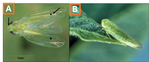
Figure 1. Cotton jassid adults (A) have one black dot on each wing and may have two small dots between their eyes (these dots on the crown can fade). The potato leafhopper (B), which is not a threat to cotton production but does occur in Oklahoma, does not have black dots on their wings or between their eyes. Image A courtesy of Isaac Esquivel, UF Extension, image B courtesy of DryBeanAgronomy.ca.
Biology and Host Range
The cotton jassid has a short life cycle, completing a generation in approximately two weeks under warm conditions.
- Reproduction: Eggs are inserted directly into leaf midveins and petioles, hatching in 3–4 days. Eggs will not be visible to the naked eye or through hand lens. Cotton jassids progress through 5 nymphal instars before becoming reproductive adults (Figure 2).
- Host Plants: This pest is polyphagous, meaning it feeds on many hosts. While cotton is a primary target, it also thrives on okra, eggplant, and ornamental hibiscus. It has also been found on native plants like Turk’s cap, as well as weeds like Ceasar weed and Florida pusley.
- 2025 Range on U.S. Cotton: The cotton jassid was detected on cotton in FL, GA, AL, MS, LA, TN, SC, NC, and TX. The TX detections in cotton were limited to southeastern TX in Grimes, Wharton, and Fort Bend counties. At the time of this article’s posting (March 2026), the cotton jassid has not been detected in OK.
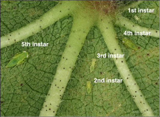
Figure 2. Cotton jassid nymphs on the underside of a cotton leaf. Image courtesy of Isaac Esquivel, UF Extension.
Damage: Recognizing Hopperburn
Unlike other leafhoppers, the cotton jassid injects a salivary toxin that disrupts the plant’s vascular system.
- Early Signs: Initial yellowing that resemble potassium deficiency with some upward curling of leaf margins (Figure 3, Rating 1).
- Progression: Characterized by hopperburn, a yellowing (chlorosis) that proceeds from leaf edges and turns red or brown as the tissue dies (Figure 3).
- Systemic Impact: Plants can go downhill quickly, often leading to complete desiccation and stunted growth (Figure 4).
A Hopperburn Injury Rating Scale has been developed by Extension Cotton Entomologists in the mid-South (Figure 3). You cannot let the cotton jassid get ahead of you. Once reddening starts on the leaf margins (Rating 2 in Figure 3) it is likely too late to rescue the cotton plant, damage will quickly progress and photosynthetic capabilities for the plant decline considerably.
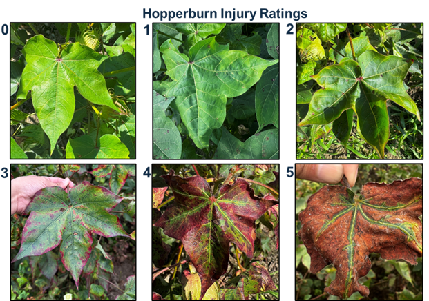
Figure 3. Hopperburn injury rating scale for cotton jassid damage. Damage increases from none (0) to severe damage of desiccated leaf (5). Slight yellowing and upward curling of leaf is shown in Rating 1, with increased yellowing, cupping, and beginnings of reddened leaf margins in Rating 2. Insecticide action should be taken prior to reaching Rating 2. Ratings 3 – 5 show increased spread of reddening and desiccation. Images courtesy of Phillip Roberts (UGA Extension) and Scott Graham (AU Extension).
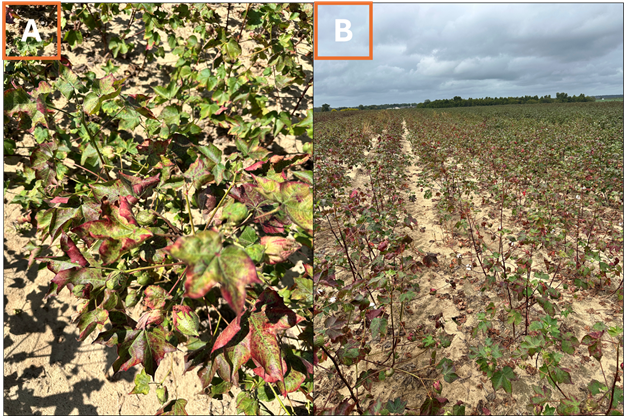
Figure 4. Cotton jassid hopperburn resulting in reddened, dried leaves (A) and stunted cotton plants (B). Image courtesy Isaac Esquivel, UF Extension.
Scouting Protocol
Scouting is mandatory for every cotton field in 2026 to prevent significant yield loss. Plants located at the edge of cotton fields can serve as good indicators, as cotton jassids will enter at field margins where damage is more likely to occur before further in field.
- Target Area: Inspect the undersides of leaves in the mid-to-upper canopy.
- Sample Leaf: Focus on the 4th mainstem leaf below the terminal, as this is where nymphs typically congregate.
- Visual Checks: Because adults fly quickly, count the flightless nymphs. Examine at least 25 leaves per field.
- Threshold: 1 cotton jassid per leaf, or early crop injury indicators (Figure 3, Rating 1) with cotton jassid confirmations nearby.
- Continue Scouting: Since green leaves are needed to fill bolls, growers should scout cotton up to at least 2 weeks prior to defoliation.
Management Guidance
Cultural Practices
- Plant Early: Trials indicate that earlier planting dates can help the crop “outrun” the peak pressure of migrating populations.
- Nutrient Management: Avoid excess Nitrogen, which attracts cotton jassids. Ensure adequate Potassium, as deficient plants crash much faster under cotton jassid stress.
- Varieties: Internationally, varieties with high trichome (hair) density on leaves offer natural resistance to feeding. However, varieties on the U.S. market are generally less hairy than those planted elsewhere. Currently, trials from 2025 do not indicate a varietal difference in terms of cotton jassid susceptibility.
Chemical Control
Based on 2025 research trials conducted by Mid-South Cotton Extension Entomologists, the following insecticides have shown varying levels of control (Table 1). Repeated insecticide applications may be warranted.
Table 1. Suggested foliar insecticides* and their observed control level for suppressing the cotton jassid. Efficacy lasted around 2 weeks.
| Control Level | Insecticides |
| High (>70% Control) | Carbine, Sefina, Sivanto, Bidrin, Venom, Plinazolin |
| Moderate (50-70%) | Transform, Centric, Assail, Orthene |
| Low (<50%) | Steward, Diamond, Bifenthrin, Admire Pro |
*Cotton jassids have shown resistance to every chemistry class in their native range; rotation of modes of action is critical. The mention, listing, or use of specific insecticides is not an endorsement of that product, nor is it a criticism of similar products not mentioned.
If you suspect cotton jassid activity or see hopperburn symptoms, contact the OSU Cotton IPM team: Maxwell Smith (maxwell.smith@okstate.edu), Ashleigh Faris (Ashleigh.faris@okstate.edu), and Jenny Dudak (jdudak@okstate.edu) immediately for confirmation. This team will be monitoring for the cotton jassid and will share updates on nearing threat, Oklahoma detections, and updated management guidance as it becomes available.
For more information on the cotton jassid in the U.S., click on this link to access Extension Factsheets, podcasts, and videos developed by Extension Entomologists managing the pest: https://drive.google.com/file/d/19IFT5c9b5JXEaBgf6X-weya07G56RXS5/view?usp=sharing.
Brown Wheat Mite Activity in North Central Oklahoma
Ashleigh Faris, Cropping Systems Entomologist, IPM Coordinator
Department of Entomology & Plant Pathology,
Oklahoma State University
Following a period of dry weather, wheat growers in central Oklahoma are reporting activity of the Brown Wheat Mite (BWM). Unlike many other wheat pests, BWM thrives in drought conditions, and its damage can often be mistaken for moisture stress or nutrient deficiency.
Identification
The Brown Wheat Mite is small—about the size of a needle point—but is generally easier to spot than the Wheat Curl Mite because it is active on the leaf surface.
- Appearance: BWM has a dark red to brownish-black, oval-shaped body (Figure 1).
- Distinguishing Feature: Its front legs are significantly longer than its other three pairs of legs.
- Behavior: They are most active during the day, particularly in the afternoon, and will quickly drop to the ground if the plant is disturbed (Figure 2).
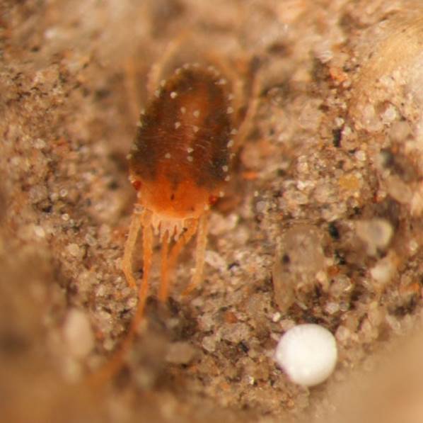
Figure 1. Brown wheat mite (BWM).
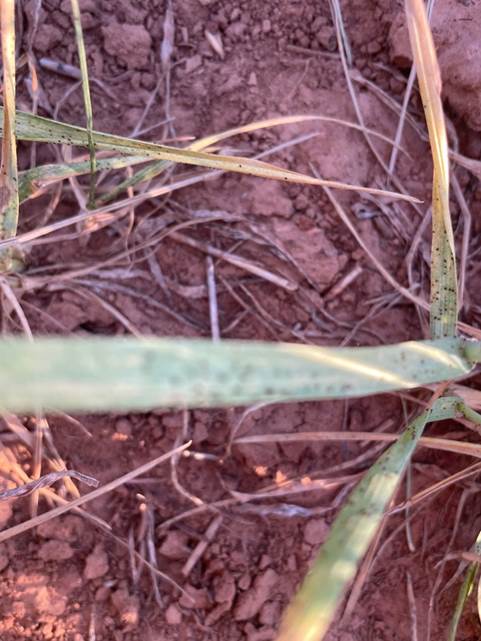
Figure 2. Brown wheat mites (BWM) on wheat. Image courtesy L. Galvin, OSU Extension.
Biology and Life Cycle
BWM populations consist entirely of females that produce offspring without mating (parthenogenesis), allowing for extremely rapid population growth under dry conditions. The BWM has a unique life cycle in that it can lay two types of eggs. Environmental conditions dictate when these two types of eggs are laid:
- Red Eggs: Laid during the growing season and hatch in about a week when conditions are favorable.
- White (Diapause) Eggs: Laid as temperatures rise and the crop matures. They are highly resistant and allow the population to survive the summer heat, hatching only when cooler, wetter weather arrives in the fall.
Damage
BWM damage is caused by the mites piercing plant cells and sucking out the plant nutrients.
- Symptoms: Initial damage appears as “stippling” (fine white or yellow spots) on the leaves. As feeding continues, leaves take on a silvery or bronzed appearance (Figure 3).
- Tipping: Heavy infestations cause the tips of the leaves to turn brown and die.
- Weather Interaction: Damage is most severe when plants are already under drought stress. Because both BWM damage and drought cause yellowing/browning, it is essential to confirm the presence of mites before treating.
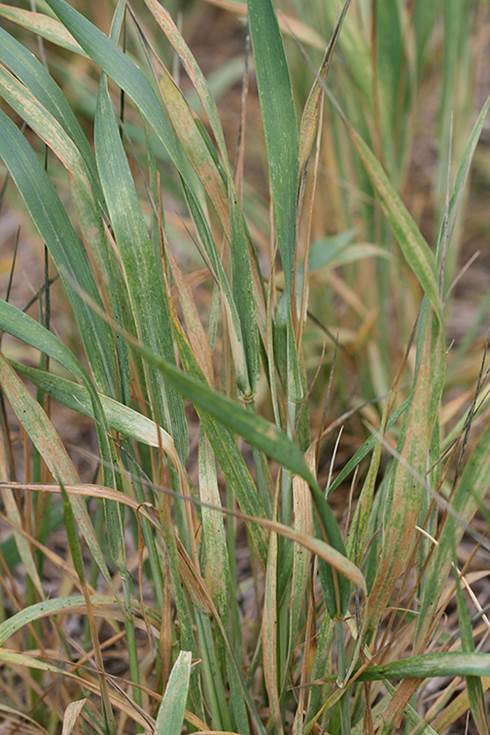
Figure 3. Brown wheat mite (BWM) damage.
Scouting
Because BWM is highly mobile and drops when disturbed, careful scouting is required:
- Timing: Scout during the warmest part of the day when mites are most active on the upper leaves.
- The Paper Test: Gently but quickly shake or tap wheat plants over a white piece of paper or a white clipboard. Look for tiny dark specks moving across the surface.
- Economic Threshold: While thresholds vary based on crop value and moisture stress, research suggests a treatment threshold of 25 to 50 brown wheat mites per leaf in wheat that is 6 inches to 9 inches tall is economically warranted. An alternative estimation is “several hundred” per foot of row. If the wheat is severely stressed, the lower end of that threshold should be used.
Management Recommendations
- The “Rain” Factor: A significant, driving rain is often the most effective control for BWM. Rain can physically knock mites from the plant and promote fungal pathogens that naturally reduce the population.
- Chemical Control: If populations exceed the threshold and no rain is in the forecast, chemical intervention may be necessary. Know the cost of the treatment and value of your wheat so you can determine if an application is a worth return on investment.
- Effective Ingredients: Organophosphates (such as Dimethoate) have historically provided better control than many pyrethroids, as the latter can sometimes result in mite “flaring” or simply fail to provide adequate residual control.
- Coverage: High water volume is critical to ensure the insecticide reaches the mites, especially if they have moved toward the base of the plant.
- Pre-harvest Intervals & Grazing Restrictions: Always read and follow the label guidelines. For more on acaricides that can be applied in wheat see the Oklahoma State University Fact Sheet “Management of Insect and Mite Pests in Small Grains” (CR-7194).
- Cultural Practices: Since BWM thrives in dry, dusty conditions, maintaining good soil moisture and vigorous plant growth can help the crop tolerate feeding. Here’s to hoping for some rain soon in the forecast; we could really use it for lots of reasons in Oklahoma.
Check Your Wheat: Greenbugs Reported in Central Oklahoma
Ashleigh M. Faris
Cropping Systems Extension Entomologist
Department of Entomology & Plant Pathology
Oklahoma State University
Wheat producers in central Oklahoma are reporting the presence of the greenbug, Schizaphis graminum, in winter wheat fields. Greenbugs are one of the most important insect pests of wheat in the southern Great Plains and can occur from fall through spring. These aphids feed on plant sap and inject toxins into wheat plants, causing characteristic leaf discoloration and plant injury.
Early detection through field scouting is essential to determine whether populations are increasing and if an insecticide treatment is justified.
Greenbug Identification & Biology
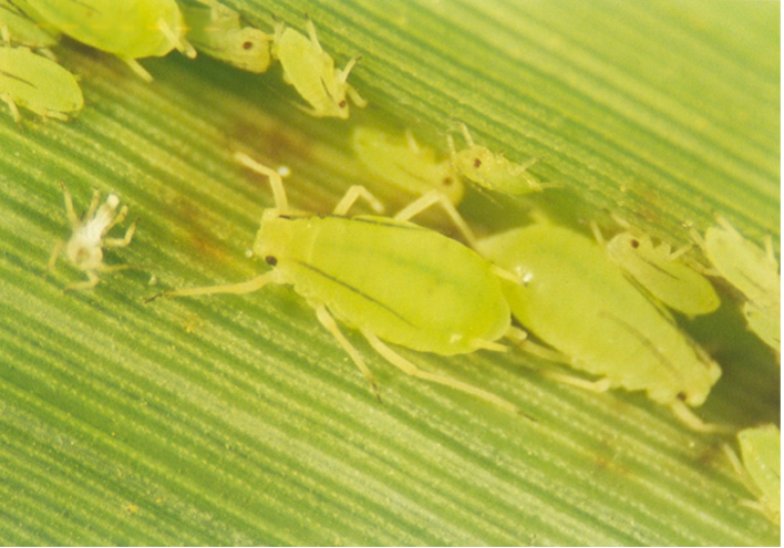
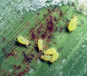
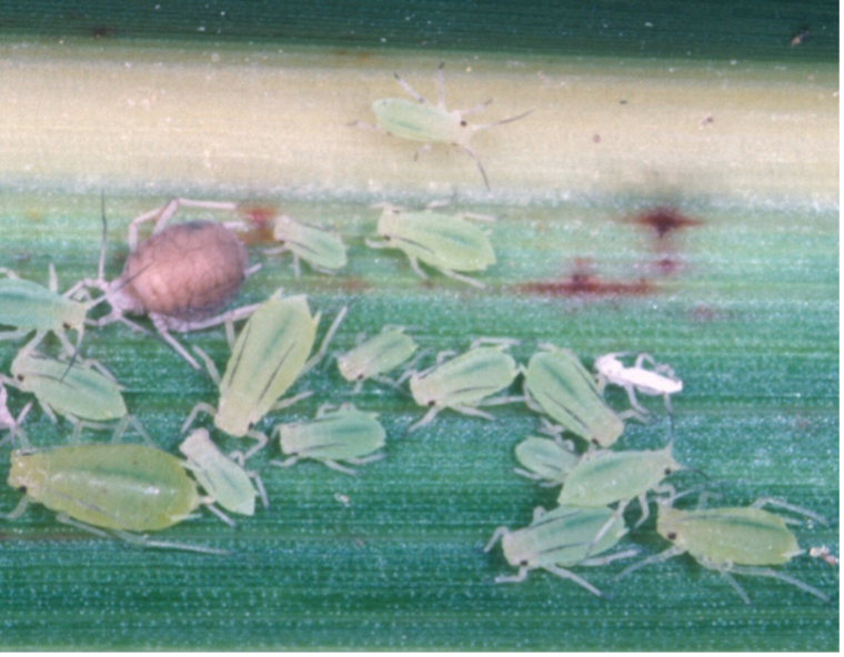
Key identifying characteristics of greenbug (Figure 1):
- Small aphids (~1/16 inch long)
- Pale to lime-green body
- Dark green stripe down the middle of the back
- Dark tips on antennae and legs
- Found in colonies on the underside of wheat leaves
Greenbugs reproduce rapidly under favorable conditions (between 55° F and 95° F) and often occur in patches within fields rather than evenly distributed populations. During periods of cool weather, the greenbug may increase to enormous numbers, due to the absence of natural enemies, which develop significantly slower compared to greenbugs at such temperatures. On the other hand, cold weather can also influence aphid populations. However, this latest cold snap is not enough to eliminate greenbugs. It takes average temperatures below 20° F for at least a week to kill a substantial number of greenbugs in wheat.
Greenbug Damage in Wheat
Greenbugs damage wheat in two ways, through direct feeding and injection of toxic saliva. Greenbugs may also transmit barley yellow dwarf virus (BYDV), which can further reduce yield potential.
Typical early symptoms include small, reddish or copper spots on leaves (Figure 2) and yellowing around feeding sites. Advanced infestations will result in leaves turning yellow or orange, dead leaf tissue, stunted plants, and expanding patches of dead wheat. Heavy infestations may kill seedlings and reduce tillering, particularly during drought stress.
How to Scout for Greenbugs
The Glance-N-Go™ sampling system developed by Oklahoma State University can help determine whether aphid populations exceed economic thresholds. Download the Greenbug Glance N’ Go Sampler app for your smartphone. You will then input the control cost ($/Acre), crop value ($/Acre), and the Spring sampling window. Use a zig-zag or W-pattern (Figure 3) to scout your field, checking undersides of leaves at three tillers per stop for greenbugs and brown mummies. Use the app to record the numbers of these insects and sample until the app tells you to stop sampling or tells you treat. As temperatures warm, continue to scout regularly as greenbug populations may build.

Scouting recommendations without the Greenbug Glance N’ Go Sampler app:
- Walk a W or zigzag pattern across the field.
- Examine 10–20 plants at each stop.
- Check:
- Underside of leaves
- Leaf midrib
- Base of tillers
- Record:
- Aphids per tiller
- Presence of aphid mummies (Figure 4)
- Beneficial insects
Beneficial Insects
Natural enemies frequently control aphid populations. While scouting for greenbug you should also look for lady beetles, lacewing larvae, hoverfly larvae, and parasitized aphids (“mummies”) (Figure 4). If beneficial insects are abundant, aphid populations may decline without insecticide treatment. Where there are one to two lady beetles (adults and larvae) per foot of row, or 15 to 20 percent of the greenbugs have been parasitized, control measures could be delayed until it is determined whether the greenbug population is continuing to increase.
Based on current wheat scouting, it appears that parasitoid numbers are low this 2026 season so continuing to scout for greenbug will be critical in responding to populations that go unchecked by beneficials.
Economic Threshold Guidelines
The simplest way to determine if action needs to be taken against greenbugs is to utilize the Glance-N-Go™ sampling system developed by Oklahoma State University. Approximate guidelines historically used in Oklahoma wheat can be found in Table 1 below.
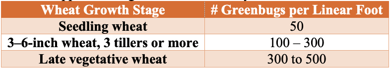
Thresholds are influenced by:
- Wheat growth stage
- Crop value
- Cost of treatment
- Presence of beneficial insects
Insecticides Labeled for Greenbugs in Wheat
Aphid feeding and insecticide performance are strongly influenced by temperature. Greenbugs tend to move higher on wheat plants during warm conditions but may move lower on the plant or below ground during cold weather, reducing exposure to insecticides. As a result, damaging populations are most often observed in late winter and early spring. Insecticides generally perform best when temperatures are above 50°F, and control may occur more slowly in cooler conditions (e.g., control at 45° F may take roughly twice as long as at 70° F). If applications must be made under cooler temperatures, use the highest labeled rate. Wheat grown under irrigation can typically tolerate higher greenbug populations than dryland wheat.
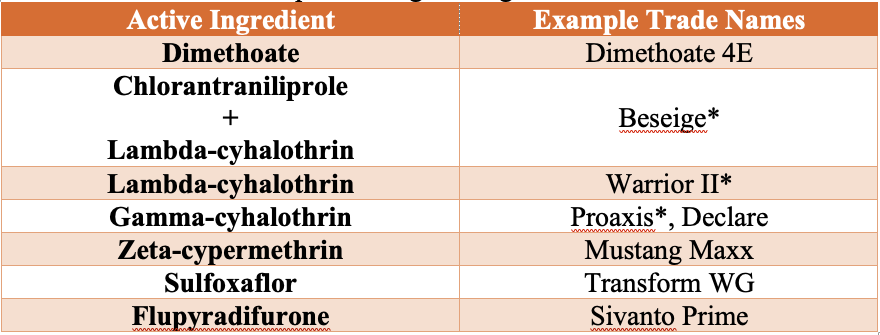
Always follow pesticide label directions, application sites, and rates. Be sure to read and follow the label for preharvest intervals (PHI) and restricted-entry intervals (REI). Use a minimum of 10 GPA by ground and 3 GPA by air (if labelled for aerial application) to ensure adequate coverage.
For assistance with aphid identification or treatment decisions, see OSU Fact Sheet EPP-7099 Small Grain Aphids in Oklahoma and Their Management, or contact your local OSU Extension office.
Thoughts from an Agronomist- 1 Management of the Primordia
Josh Lofton, Cropping Systems Specialist
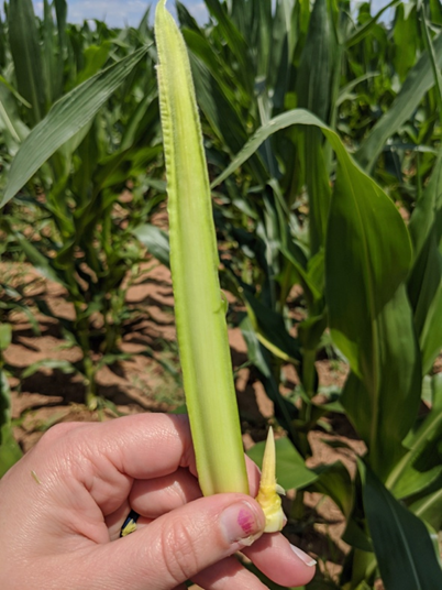
Many crop management recommendations emphasize actions that must be taken well before a crop reaches what we often call “critical growth stages.” Management this early can seem counterintuitive when the crop still looks small, healthy, or unchanged aboveground. However, much of a crop’s yield potential is determined early in the season at a level we cannot see in the field. Long before flowers, tassels, or heads (or any reproductive structure) appear, the plant is already making developmental decisions that shape its final yield potential. Understanding this “behind the scenes” process helps explain why timely, early-season management is often more effective than trying to correct problems later.
At the center of this process is the shoot apical meristem, commonly referred to as the growing point. This tissue produces leaf and reproductive primordia, which are the earliest developmental stages of future everything in the plant. These primordia form well before the corresponding plant parts are visible. Once these structures initiate—or if they fail to begin due to stress—the outcome is permanent. The plant cannot later in the season go back and recreate leaf number, leaf size, or reproductive capacity. As a result, early environmental conditions and management decisions play a disproportionate role in determining yield potential.
Corn is a good example of how early development influences final yield. By the time corn reaches the V4 growth stage, the plant only has four visible leaves with collars, yet internally it is far more advanced. Most of the total leaf primordia that will eventually form the full canopy have already begun, and the potential size of the ear is starting to be established. During this stage, the growing point is still below the soil surface and somewhat protected from some stressors but highly susceptible to others. Nitrogen deficiency, cold temperatures, moisture stress, compaction, or herbicide injury at or before V4 can reduce leaf number and limit leaf expansion. Even if growing conditions improve later, the plant cannot replace leaf primordia that were never formed, which reduces its ability to intercept sunlight and support high yields.
As corn approaches tasseling (VT), the crop enters a stage that is visually and physiologically important. Pollination, fertilization, and early kernel development occur at this time, and stress can have a critical impact on kernel set. However, by VT, the plant has already completed leaf formation, and much of the ear size potential has already been determined several growth stages earlier. Management at VT is therefore focused on protecting yield rather than creating it. Late-season nutrient applications may improve plant appearance or maintain green leaf area, but they cannot increase leaf number or rebuild ear potential lost due to early-season stress. This distinction helps explain why some late inputs show limited yield response even when the crop looks responsive.
Grain sorghum provides another clear example of why early management is emphasized. Although sorghum often grows slowly early in the season and may appear unimportant during the first few weeks after emergence, the first 30 days are among the most critical periods in its development. During this time, the growing point is actively producing leaf primordia and transitioning from vegetative growth toward reproductive development. Head size potential is primarily established during this early window, and the plant’s capacity to support tillers is influenced by early nutrient availability and moisture conditions. Stress from nitrogen deficiency, drought, weed competition, or restricted rooting during the first 30 days can reduce head size and kernel number long before visible symptoms appear.
Once sorghum reaches later vegetative and reproductive stages, much like corn at VT, management shifts from building yield potential to protecting what has already been determined. Improving conditions later in the season can help maintain plant health and grain fill, but it cannot fully compensate for early limitations imposed at the primordial level. This is why early fertility placement, timely weed control, and moisture conservation are consistently emphasized in sorghum production systems.
Across crops, a typical pattern emerges: the growth stages we observe in the field often reflect decisions the plant made weeks earlier. When agronomists stress early-season management, they are responding to plant biology rather than simply following tradition. By the time visible “critical stages” arrive, the plant has already established many of the components that define yield potential.
The key takeaway is that effective crop management must be proactive rather than reactive. Early-season decisions support the crop while it is still determining how many leaves it can produce, how large its reproductive structures can become, and how much yield it can ultimately support. Waiting until stress becomes visible often means responding after the plant has already adjusted its potential downward. Recognizing what is happening at the primordial level helps explain why management ahead of critical stages consistently delivers the greatest return, even when the crop appears small and unaffected aboveground.
For questions or comments reach out to Dr. Josh Lofton
josh.lofton@okstate.edu
Cotton disease update: Reniform nematode – 08/25/2025
Maíra Duffeck, OSU Row Crops Extension Pathologist, Department of Entomology and Plant Pathology Oklahoma State University
Maxwell Smith, OSU IPM for Cotton Extension Specialist, Department of Entomology and Plant Pathology, Oklahoma State University
Jenny Dudak, OSU Extension Cotton Specialist, Department of Plant & Soil Sciences Oklahoma State University
Reniform nematode continues to be detected in cotton fields across Oklahoma. During the 2023 and 2024 growing seasons, a survey was conducted in 17 commercial cotton fields located in Tillman, Jackson, Grady, and Caddo counties to assess the presence of parasitic nematodes affecting cotton production. We collected soil samples in areas of the fields showing irregular and stunted cotton plants.
Out of the 17 soil samples collected, reniform nematode was detected in 5 fields, marking the first confirmed report of this pest in Oklahoma cotton. Notably, in one of the positive fields, the reniform nematode population reached 1,569 nematodes per 100 cm³ of soil; more than double the economic threshold of 700 nematodes per 100 cm³. In 2025, a soil sample from a cotton field in Jackson County already tested positive for the reniform nematode.
The reniform nematode, caused by Rotylenchulus reniformis, is one of the most important yield-limiting pathogens of cotton production in the southern U.S. In addition to cotton, the reniform nematode can reproduce on other field crops such as soybean, with yield loss estimates being greater in cotton than soybean. The reniform nematode is easy to introduce into new fields because of its unique ability to survive in a dehydrated state in dry soils. Therefore, it can be transported long distances on field equipment.
We suspect that parasitic nematodes, such as root-knot and reniform nematodes, are already present in many Oklahoma cotton fields, but the damage they cause often goes unnoticed. This is especially important for the reniform nematode, as yield losses can occur without obvious aboveground symptoms. For this reason, monitoring the distribution of this nematode across the cotton fields in Oklahoma is crucial to raise awareness of this emerging issue and to guide future management decisions.
Symptoms and Signs
The expression of symptoms depends on several factors, including the susceptibility of the cotton hybrid, nematode population levels, soil type, and for how long that field has been infested. Affected plants may show reduced growth, delayed flowering, fewer fruits, and smaller fruit size, which together contribute to yield losses in lint or pods. Unlike the southern root-knot nematode (Meloidogyne incognita), the reniform nematode does not induce gall formation on roots, making field diagnosis based solely on visible symptoms challenging. For this reason, soil testing through a nematode assay is often necessary for proper identification. In newly infested fields, stunted plants are typically the most noticeable sign (Figure 1).
Plan of Action
To address this issue, a statewide nematode survey is underway to document the presence, abundance, and geographic distribution of parasitic nematodes in Oklahoma cotton fields. The information generated from this survey will provide a foundation for developing and implementing economically viable strategies to manage this issue and protect cotton production in the state.
How to participate?
Oklahoma cotton growers interested in having their fields tested for parasitic nematodes have several ways to participate in this study:
- Schedule a field visit: Contact Dr. Maira Duffeck to arrange soil sample collection. She can be reached by phone at 347-205-2180 or by email at mairodr@okstate.edu.
- Drop off samples at the Peanut & Cotton Field Day: September 18, 2025, from 5:00–8:00 p.m. at the Caddo Research Station (28054 County Street 2540, Ft. Cobb)
- Drop off samples at the Cotton Field Day: September 25, 2025, from 8:30 a.m. to 1:00 p.m. at the Southwest Research & Extension Center (16721 US Hwy 283, Altus)
More information about dropping off samples on OSU field days can be found on the flyers shown in Figures 2 and 3. Growers can submit soil samples for analysis at no cost, as expenses are covered through a project funded by the Oklahoma Cotton Council in partnership with Cotton Incorporated.
How to collect soil samples for analysis?
- Soil samples should be collected from the root zone of the plants
- Collect 15–20 soil cores (6–8 inches deep) from across the field
- Growers should focus on areas of the field where plants are showing poor growth and development
- Mix the cores thoroughly, then place the mixed soil into a resealable plastic bag
- We need about 2 pints (1 kg) of soil for analysis
- Keep samples cool — store them in a refrigerator until the field day.
- If you collect soil samples from different fields, please label and add field information to the plastic bag accordingly


For Additional Information contact.
Dr. Maíra Duffeck mairodr@okstate.edu
Toto, I’ve a feeling we’re not in Kansas anymore. Double Cropping, Orange edition
It has been pointed out that the blog https://osunpk.com/2025/06/09/double-crop-options-after-wheat-ksu-edition/ had a significant Purple Haze. And I should have added the Oklahoma caveat. So Dr. Lofton has provided his take on DC corn in Oklahoma.
Double-crop Corn: An Oklahoma Perspective.
Dr. Josh Lofton, Cropping Systems Specialist.
Several weeks ago, a blog was published discussing double-crop options with a specific focus on Kansas. I wanted to address one part of that blog with a greater focus on Oklahoma, and that section would be the viability of double-crop corn as an option.
Double-crop farming is considered a high-risk, high-reward system to try. Establishing a crop during the hottest and often driest parts of summer can present challenges that need to be overcome. Double-crop corn faces these same challenges and, in some seasons, even more. However, it is definitely a system that can work in Oklahoma, especially farther south. If you look at that original blog post, one of the main challenges discussed is having enough heat units before the first frost. When examining historic data, like those below from NOAA, the first potential frost date for Northcentral and Northwest Oklahoma may be as early as the first 15 days of October but more often will be in the last 15 days of October. In Southwest and Central Oklahoma, this date shifts even later to the first 15 days of November. This is later than Kansas, especially northern Kansas, which has a much higher chance of experiencing an early October freeze. I do not want to downplay this risk; however, it is one of the biggest risks growers face with this system, and a later fall freeze would greatly benefit it. We have been conducting trials near Stillwater for the past five years on double-crop corn and have only failed the crop once due to an early freeze event. But in that year, both double-crop soybean and sorghum also did not perform well.

The main advantage of double-crop corn is that if you miss the early season window, it offers the best chance for the crop to reach pollination and early grain fill without the stress of the hottest and driest part of the year. Therefore, careful management is crucial to ensure this benefit isn’t lost. In Oklahoma, we have two systems that can support double-crop corn. In more central and southwest Oklahoma, especially under irrigation, farmers can plant corn soon after wheat harvest, similar to other double-crop systems. This planting window helps minimize the impact of Southern Rust, which can significantly reduce yields in some years, and may reduce the need for extensive management. This earlier planting window is often supported by irrigation, enabling the crop to endure the hotter, drier late July and early August periods. Conversely, in northern Oklahoma, planting often occurs in July to allow pollination and grain fill (usually 30-45 days after emergence) to happen in late August and early September. During this period, the chances of rainfall and cooler nighttime temperatures increase, both of which are critical for successful corn production.
Other management considerations include maturity. Based on initial testing in Oklahoma, particularly in the northern areas, we prefer to plant longer-maturity corn. Early corn varieties have a better chance of maturing before a potential early freeze but also carry a higher risk of undergoing critical reproduction stages (pollination and early grain fill) during hot, dry periods in late summer. Testing indicates that corn with a maturity of over 110 days often works well for this. However, this does not mean growers cannot plant shorter-season corn, especially if the season has generally been cooler, though the risk still exists depending on how quickly the crop can grow. Based on testing within the state, the dryland double-crop corn system typically does not require adjustments to other management practices, such as seeding rates or nitrogen application. Because of the need to coordinate leaf architecture and manage limited water resources, higher seeding rates are not recommended. Maintaining current nitrogen levels allows the crop to develop a full canopy.
The final question often comes as; how does it yield? This will depend greatly. Corn looks very good this year across that state, especially what was able to be planted earlier in the spring. However, in recent years, delaying even a couple of weeks beyond traditional planting windows has lowered yields enough that double-crop yields are often similar. We have often harvested between 50-120 bushels per acre in our plots around Stillwater with double-crop systems. So, the yield potential is still there.
In the end, Oklahoma growers know that double-crop is a risk regardless of the crop chosen. There are additional risks for double-crop corn, such as Southern Rust in the south and freeze dates in the north. This risk is increased by the presence of Corn Leaf Aphid and Corn Stunt last season, and it is not clear if these will be ongoing problems. Therefore, growers need to be careful not to expect too much or to invest too heavily in inputs that may not be recoverable if there is a loss. One silver lining is that if double-crop corn doesn’t succeed in any given year, growers can still use it as forage and recover at least some of their costs.
Any questions or concerns reach out to Dr. Lofton: josh.lofton@okstate.edu
Army Worms are Marching!!!!
This article by Brian Pugh (new OSU State Forage Specialist) just came across my desk today in perfect timing as yesterday I saw significant army worm feeding on the crabgrass in my lawn, and not to mention the 20+ caterpillars on my sidewalk. So while Brian is noting Eastern Ok, Id say we are at thresholds in Payne Co also. And no, we don’t need to discuss that my lawn as more crabgrass than Bermuda.
Fall Armyworms Have Arrived In Oklahoma Pastures and Hayfields
Brian C. Pugh, Forage Extension Specialist
Fall armyworms (FAW) are caterpillars that directly damage Bermudagrass and other introduced forage pastures, seedling wheat, soybean and residential lawns. There have been widespread reports of FAW buildups across East Central and Northeast Oklahoma in the first two weeks of July. Current locations exceeding thresholds for control are Pittsburg, McIntosh and Rogers counties.

Female FAW moths lay up to 1000 eggs over several nights on grasses or other plants. Within a few days, the eggs hatch and the caterpillars begin feeding. Caterpillars molt six times before becoming mature, increasing in size after each molt (instars). The first instar is the caterpillar just after it hatches. A second instar is the caterpillar after it has shed its skin for the first time. A sixth instar has shed its skin five times and will feed, bury itself in the soil, and pupate. The adult moth will emerge from the pupa in two weeks and begin the egg laying process again after a suitable host plant is found. Newly hatched larvae are white, yellow, or light green and darken as they mature. Mature FAW measure 1½ inches long with a body color that ranges from green, to brown to black.

Large variation in color is normal and shouldn’t be used alone as an identifying characteristic. They can most accurately be distinguished by the presence of a prominent inverted white “y” on their head. However, infestations need to be detected long before they become large caterpillars. Small larvae do not eat through the leaf tissue, but instead, scrape off all the green tissue and leave a clear membrane that gives the leaf a “window pane” appearance. Larger larvae however, feed voraciously and can completely consume leaf tissue.

FAW are “selective grazers” and tend to select the most palatable species of forages on any given site to lay eggs for young larvae to begin feeding. The caterpillars also tend to feed on the upper parts of the plant first which are younger and lower in fiber content. Forage stands that are lush due to fertility applications are often attacked first and should be scouted more frequently.

To scout for FAW, plants from several locations within the field or pasture need to be examined. Examine plants along the field margin as well as in the interior. Look for “window paned” leaves and count all sizes of larvae. OSU suggests a treatment threshold is two or three ½ inch-long larvae per linear foot in wheat and three or four ½ inch-long larvae per square foot in pasture. An easy-to-use scouting aid can be made for pasture by bending a wire coat hanger into a hoop and counting FAW in the hoop. The hoop covers about 2/3 of a square foot, so a threshold in pasture would be an average of two or three ½ inch-long larvae per hoop sample. An excellent indicator plant in forage stands is Broadleaf Signalgrass (seen in the foreground of the hay bale picture). Broadleaf Signalgrass tends to be preferentially selected by female moths and is one of the first species that window paned tissue is observed during the onset of an infestation.
Approximately 70% of the forage consumed during an armyworm’s lifetime occurs in the final instar before pupating into a moth. This indicates that control measures should focus on small instar caterpillars (1/2 inch or less) before forage loss increases exponentially. Additionally, small larvae are much more susceptible to insecticide control than larger caterpillars.

Remember, FAW are actively reproducing up until a good killing frost, so don’t let your guard down. If you think you have an infestation of fall armyworm please contact your local County Extension Educator. Additionally, before considering chemical control consult your Educator for insecticide recommendations labeled for forage use.
For more information or insecticide options consult:
Oklahoma State University factsheet:
CR-7193, Management of Insect Pests in Rangeland and Pasture
https://extension.okstate.edu/fact-sheets/management-of-insect-pests-in-rangeland-and-pasture.html
Double Crop Options After Wheat (KSU Edition)
Stolen from the KSU e-Update June 5th 2025.
Double cropping after wheat harvest can be a high-risk venture for grain crops. The remaining growing season is relatively short. Hot and/or dry conditions in July and August may cause problems with germination, emergence, seed set, or grain fill. Ample soil moisture this year can aid in establishing a successful crop after wheat harvest. Double-cropping forages after wheat works well even in drier regions of the state.
The most common double crop grain options are soybean, sorghum, and sunflower. Other possibilities include summer annual forages and specialized crops such as proso millet or other short-season summer crops, even corn. Cover crops are also an option for planting after wheat (see the companion eUpdate article “Cover crops grown post-wheat for forage”).
Be aware of herbicide carryover potential
One major planting consideration after wheat is the potential for herbicide carryover. Many herbicides applied to wheat are Group 2 herbicides in the sulfonylurea family with the potential to remain in the soil after harvest. If a herbicide such as chlorsulfuron (Glean, Finesse, others) or metsulfuron (Ally) has been used, then the most tolerant double crop will be sulfonylurea-resistant varieties of soybean (STS, SR, Bolt) or other crops. When choosing to use herbicide-resistant varieties, be sure to match the resistance trait with the specific herbicide (not only the herbicide group) that you used. This is especially true when looking at sunflowers as a double crop. There are sunflowers with the Clearfield trait, which allows Beyond herbicide applications, and ExpressSun sunflowers, which allow an application of Express herbicide. While both of these herbicides are Group 2 (ALS-inhibiting herbicides), the Clearfield trait and ExpressSun are not interchangeable, and plant damage can result from other Group 2 herbicides.
Less information is available regarding the herbicide carryover potential of wheat herbicides to cover crops. There is little or no mention of rotational restrictions for specific cover crops on the labels of most herbicides. However, this does not mean there are no restrictions. Generally, there will be a statement that indicates “no other crops” should be planted for a specified amount of time, or that a bioassay must be conducted prior to planting the crop.
Burndown of summer annual weeds present at planting is essential for successful double-cropping. Assuming glyphosate-resistant kochia and pigweeds are present, combinations of glyphosate with products such as saflufenacil (Sharpen) or tiafenacil (Reviton), or alternative treatments such as paraquat may be required. Dicamba or 2,4-D may also be considered if the soybean varieties with appropriate herbicide resistance traits are planted. In addition, residual herbicides for the double crop should be applied at this time.
Management, production costs, and yield outlooks for double crop options are discussed below.
Soybeans
Soybeans are likely the most commonly used crop for double cropping, especially in central and eastern Kansas (Figure 1). With glyphosate-resistant varieties, often the only production cost for planting double crop soybeans was the seed, an application of glyphosate, and the fuel and equipment costs associated with planting, spraying, and harvesting. However, the spread of herbicide-resistant weeds means additional herbicides will be required to achieve acceptable control and minimize the risk of further development of resistant weeds.
Weed control. The weed control cost cannot really be counted against the soybeans, since that cost should occur whether or not a soybean crop is present. In fact, having soybeans on the field may reduce herbicide costs compared to leaving the field fallow. Still, it is recommended to apply a pre-emergence residual herbicide before or at planting time. Later in the summer, a healthy soybean canopy may suppress weeds enough that a late-summer post-emergence application may not be needed.
Variety selection for double cropping is important. Soybeans flower in response to a combination of temperature and day length, so shifting to an earlier-maturing variety when planting late in a double crop situation will result in very short plants with pods that are close to the ground. Planting a variety with the same or perhaps even slightly later maturity rating (compared to soybeans planted at a typical planting date) will allow the plant to develop a larger canopy before flowering. Planting a variety that is too much later in maturity, however, increases the risk that the beans may not mature before frost, especially if long periods of drought slow growth. The goal is to maximize the length of the growing season of the crop, so prompt planting after wheat harvest time is critical. The earlier you can plant, the higher the yield potential of the crop if moisture is not a limiting factor.
Fertilizer considerations. Adding some nitrogen (N) to double-crop soybeans may be beneficial if the previous wheat yield was high and the soil N was depleted. A soil test before wheat harvest for N levels is recommended. Use no more than 30 lbs/acre of N. It would be ideal to knife-in the fertilizer. If that is not possible, banding it on the soil surface would be acceptable. Do not apply N in the furrow with soybean seed as severe stand loss can occur.
Seeding rates and row spacing. Seeding rate can be slightly increased if soybeans are planted too late in order to increase canopy development. Narrow row spacing (15-inch or less) has often resulted in a yield advantage compared to 30-inch rows in late plantings. Soybeans planted in narrow rows will canopy over more quickly than in wide rows, which is important when the length of the growing season is shortened. Narrow rows also offer the benefits of increasing early-season light capture, suppressing weeds, and reducing erosion. On the other hand, the advantage of planting in wide rows is that the bottom pods will usually be slightly higher off the soil surface to aid harvest. The other consideration is planting equipment. Often, no-till planters will handle wheat residue better and place seeds more precisely than drills, although the difference has narrowed in recent years.
What are typical yield expectations for double-crop soybeans? It varies considerably depending on moisture and temperature, but yields are usually several bushels less than full-season soybeans. A long-term average of 20 bushels per acre is often mentioned when discussing double-crop soybeans in central and northeast Kansas. Rainfall amount and distribution can cause a wide variation in yields from year to year. Double-crop soybean yields typically are much better as you move farther southeast in Kansas, often ranging from 20 to 40 bushels per acre.
A recent publication explores the potential yield of double-crop soybeans relative to full-season yield (Figure 2) and the most limiting factors affecting the yields for double-crop soybeans. The link to this article is: https://bookstore.ksre.ksu.edu/pubs/MF3461.pdf.

Grain Sorghum
Grain sorghum is another double crop option. Unlike soybeans, sorghum hybrids for double cropping should be earlier maturing hybrids. Sorghum development is primarily driven by the accumulation of heat units, and the double crop growing season is too short to allow medium-late or late hybrids to mature before the first frost in most of Kansas.
Seeding rates and row spacing. Late-planted sorghum likely will not tiller as much as early plantings and can benefit from slightly higher seeding rates than would be used for sorghum planted at an earlier date. Narrow row spacing is advised, especially if the outlook for rainfall is good.
Fertilizer considerations. A key component for the estimation of N application rates is the yield potential. This will largely determine the N needs. It is also important to consider potential residual N from the wheat crop. This can be particularly important when wheat yields are lower than expected. In that situation, additional available N may be present in the soil. Assess the amount of profile N by taking soil samples at a depth of 24 inches and submitting them for analysis at a soil testing laboratory.
Double crop sorghum planted into average or greater-than-average amounts of wheat residue can result in a challenging amount of residue to deal with when planting next year’s crop. Nitrogen fertilizer can be tied up by wheat residue, so use application methods to minimize tie-up, such as knifing into the soil below the residue.
Weed control. Weed control can be important in double-crop sorghum. Warm-season annual grasses, such as crabgrass, can reduce double-crop sorghum yields. Using a chloroacetamide-and-atrazine pre-emergence product may be key to successful double-crop sorghum production. Herbicide-resistant grain sorghum varieties will allow the use of imazamox (Imiflex in igrowth sorghums) or quizalofop (FirstAct in DoubleTeam grain sorghum) that can control summer annual grasses.
No-till studies at Hesston documented 4-year average double crop sorghum yields of 75 bushels per acre compared to about 90 bushels per acre for full-season sorghum. A different 10-year study that did not have double crop planting but did compare early- and late-planting dates averaged 73 bushels per acre for May planting vs. 68 bushels per acre for June planting.
Sunflowers
Sunflowers can be a successful double crop option anywhere in the state, provided there is enough moisture at planting time to get a stand. Sunflowers need more moisture than any other crop to germinate and emerge because of the large seed. Therefore, stand establishment is important. Planting immediately after wheat harvest on a limited irrigation field can be a good fit to help with stand establishment.
Seeding rates and hybrid selection. When double-cropping sunflowers, producers should use similar seeding rates to what is typical for the area for full-season sunflowers. While full-season sunflowers can be successful in double-crop production, utilizing shorter-season hybrids can increase the likelihood of the sunflowers blooming and maturing before a killing frost.
Weed control. First, it is important to check the herbicide applications on the wheat. The rotation restriction to sunflowers after several commonly used wheat herbicides is 22-24 months.
Weed control can be an issue with double-crop sunflowers since herbicide options are limited, especially post-emergence. Thus, controlling weeds prior to sunflower planting is critical and may be complicated pre-plant restrictions for some herbicides. Planting Clearfield or ExpressSun sunflowers will provide additional post-emergence herbicide options, but ALS-resistant kochia and pigweeds still won’t be controlled. Imazamox (Beyond in Clearfield sunflower) has activity on small annual grasses as well as many broadleaf weeds, if they are not ALS-resistant.
Summer annual forages
With mid-July plantings, and where herbicide carryover issues are not a concern, summer annual sorghum-type forages are also a good double crop option. A study planted July 21, 2008 near Holton, when summer rainfall was very favorable, provided yields of 2.5 to 3 tons dry matter/acre for hybrid pearl millet and sudangrass at the low end to 4 to 5 tons dry matter/acre for forage sorghum, BMR forage sorghum, photoperiod sensitive forage sorghum, and sorghum x sudangrass hybrids. Earlier plantings may produce even more tonnage, as long as there is adequate August rainfall.
One challenge with late-planted summer annual forages is getting them to dry down when harvest is delayed until mid- to late-September. Wrapping bales or bagging to make silage are good ways to deal with the higher moisture forage this late in the year.
Corn
Is double-crop corn a viable option? Corn is typically not recommended for late June or July plantings because yield is usually substantially less than when planted earlier.
Typically, mid-July planted corn struggles during pollination and seldom receives sufficient heat units to fill grain before frost. Very short-season corn hybrids (80 to 95 RM) have the greatest chance of maturing before frost in double crop plantings, but generally have less yield potential when compared to hybrids of 100 RM or more used for full-season plantings. Short-season hybrids often set the ear fairly close to the ground, increasing the harvest difficulty. Glyphosate-resistant hybrids will make weed control easier with double crop corn, but problems remain present with late-emerging summer weeds such as pigweeds, velvetleaf, and large crabgrass. Keep in mind, corn is very susceptible to carryover of most residual ALS herbicides used in wheat.
Considerations for altering seeding rates and variety/hybrid maturity for the crops discussed above are summarized in Table 1.
Table 1. Seeding rate and variety/hybrid relative maturity considerations for double crops compared to full-season.
| Crop | Seeding rate | Relative maturity |
| ???????? Difference between double crop and full-season ???????? | ||
| Soybean | Increase | No change or longer |
| Sorghum | Increase | Shorter |
| Sunflower | No change | Shorter |
| Corn | No change | Shorter |
Volunteer wheat control
One of the issues with double cropping that is often overlooked by producers is the potential for volunteer wheat in the crop following wheat. If volunteer wheat emerges and goes uncontrolled, it can cause serious problems for nearby wheat fields in the fall as a host for the wheat streak mosaic complex of viruses [wheat streak mosaic (WSMV), High Plains disease (HPD), and triticum mosaic (TriMV)] that are transmitted by the wheat curl mite (WCM).
Volunteer wheat can generally be controlled fairly well with glyphosate or Group 1 herbicides such as quizalofop (Assure II, others), clethodim (Select Max, others), or sethodydim (Poast Plus, others), but control is reduced during times of drought stress. Atrazine can provide control of volunteer wheat in double-crop corn or sorghum, but control can be erratic depending on rainfall patterns.
For more detailed information about herbicides, see the “2025 Chemical Weed Control for Field Crops, Pastures, and Noncropland” guide available online at https://www.bookstore.ksre.ksu.edu/pubs/CHEMWEEDGUIDE.pdf or check with your local K-State Research and Extension office for a paper copy. The use of trade names is for clarity to readers and does not imply endorsement of a particular product, nor does exclusion imply non-approval. Always consult the herbicide label for the most current use requirements.
To Subscribe to the KSU Agronomy E-Updates follow this link
https://eupdate.agronomy.ksu.edu/index_new_prep.php
Authors contributing to the post
Sarah Lancaster, Weed Management Specialist
slancaster@ksu.edu
John Holman, Cropping Systems Agronomist
jholman@ksu.edu
Logan Simon, Southwest Area Agronomist
lsimon@ksu.edu
Tina Sullivan, Northeast Area Agronomist
tsullivan@ksu.edu
Jeanne Falk Jones, Multi-County Agronomist
jfalkjones@ksu.edu
Meet the Aster Leafhopper and Learn How to Distinguish it from the Corn Leafhopper
Ashleigh M. Faris: Extension Cropping Systems Entomologist, IPM Coordinator
Release Date June 3 2025
Last year’s corn stunt disease outbreak, caused by the corn leafhopper transmitting pathogens associated with corn stunt disease, has been on everyone’s minds. Over the past few weeks, I’ve received several calls from growers, crop consultants, and industry partners concerned about leafhoppers in corn. Fortunately, none have been corn leafhoppers, the vast majority have instead been aster leafhoppers. So far, no corn leafhoppers have been reported north of central Texas. Oklahoma did not have any reports of overwintering corn leafhoppers so if we have the insect this year it will need to migrate northward from where it currently resides. For a refresher on the corn leafhopper and corn stunt disease, check out these two previously posted OSU Pest e-Alerts: EPP-25-3and EPP-23-17.
Leafhoppers in general are insects that we have had for many years in our row and field crops. But we likely did not pay attention to them or notice them until this past year due to our heightened awareness of their existence thanks to the corn leafhopper and corn stunt disease. Below is guidance on how to distinguish between the corn leafhopper and aster leafhopper. Remember, if the corn leafhopper is detected in the state, OSU Extension will notify growers, consultants, and industry partners through Pest e-Alerts and our social media channels.
Aster Leafhopper Overview
The aster leafhopper (aka six spotted leafhopper), Macrosteles quadrilineatus, is native to North America and can be found in every U.S. state, as well as Canada. This polyphagous insect feeds on over 300 host plant species including weeds, vegetables, and cereals. Like many other leafhoppers, the aster leafhopper can be a vector of pathogens that cause disease, but corn stunt is not one of them. Instead, aster leafhoppers cause problems in traditional vegetable growing operations, as well as floral production. There is currently no concern for this insect being a vector of disease in row or field crops, including corn. Check out the OSU Pest a-Alert EPP-23-1to learn more about this insect and aster yellows disease.
Aster Leafhopper versus Corn Leafhopper
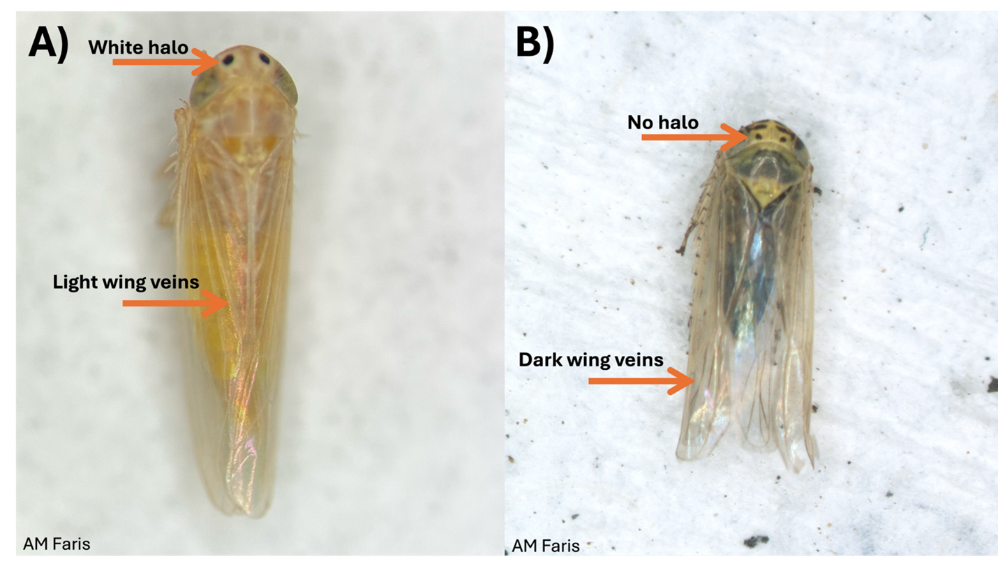
The corn leafhopper (Photo 1A) and the aster leafhopper, as well as many other leafhopper species have two black dots located between the eyes of the insect (Photo 1). Aster leafhopper adults are 0.125 inches (3 mm) long, with transparent wings that bear strong veins, and darkly colored abdomens (Photo 1B). Their dark abdomen can cause the aster leafhopper to appear grey when you see them in the field. Their long wings can also make the insect appear to have a similar appearance to the corn leafhopper (Dalbulus maidis) (Photo 1).
Characteristics that differentiate the corn leafhopper from the aster leafhopper are as follows. When viewed from above (dorsally): 1) the corn leafhopper’s dots between the eyes have a white halo around them and the aster leafhopper’s dots between eyes lack the white halo and 2) the corn leafhopper has lighter/finer wing veination than the aster leafhopper (Photo 1). When when viewed from their underside (ventrally) 3) the corn leafhopper lacks markings on their face whereas the aster leafhopper has lines/spot on the face and 4) the abdomen of the corn leafhopper lacks the dark coloration of the aster leafhopper (Photo 2).

Confirming Corn Leafhopper Identification
It is important to note that many insects will have their cuticle darken as they age. This, along with there being light and dark morphs of many insects can lend to additional confusion when distinguishing one species from another. If you believe that you have a corn leafhopper then you need to collect the insect and send it to a trained entomologist that can verify the identity of the insect under the microscope. Leafhoppers in general are fast moving insects but they can be collected in an insect net or using a handheld vacuum (see EPP-25-3). You can submit samples to the OSU Plant Disease and Insect Diagnostic Lab.
Please feel free to reach out to OSU Cropping Systems Extension Entomologist Dr. Ashleigh Faris with any questions or concerns. @ ashleigh.faris@okstate.edu
