
OSUNPK Fertilizer Market Outlook: Nitrogen Eases While Phosphate Holds Firm
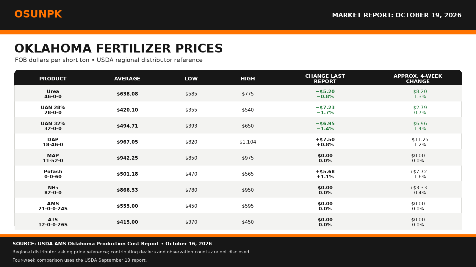
Oklahoma’s latest fertilizer report shows nitrogen moving lower while phosphorus remains firm. UAN 28% declined $7.23 per ton and UAN 32% declined $6.95 in USDA’s October 16 release. Urea also eased, while DAP increased $7.50. These are modest changes, but the different directions matter when comparing products and planning fall purchases.
Price-source note: The graphic’s Oklahoma average, minimum, and maximum come from the USDA AMS Oklahoma Production Cost Report. USDA does not identify contributing dealers. Named public dealer cash quotes, including Two Rivers, and confidential local survey observations are tracked separately and are not blended into USDA statistics.
International nitrogen news provides some context for the softer local values. Financial Express reported October 18 that India’s September landed urea cost was about $392 per metric tonne, compared with $947 at the May peak, citing improved supply and diversified sourcing. Those figures describe Indian imports, not an Oklahoma retail offer. They nevertheless show that global nitrogen supply can improve while individual local products remain expensive. Inland freight, inventory purchased earlier, product form, and the timing of replacement loads can all delay the local response.
Phosphate faces a different set of pressures. In October 8 commentary, StoneX described disruption to ammonia and sulfur supplies as a constraint on phosphate manufacturing costs. Both materials are important production inputs, so weaker demand for finished DAP or MAP does not automatically remove the cost of making the next ton. That is consistent with the local split: nitrogen solutions declined, but Oklahoma DAP increased and MAP held steady. This is an interpretation of the combined evidence, rather than proof of what drove each reporting dealer’s price.
In an October 15 IL Corn interview, fertilizer analyst Josh Linville emphasized that international supply conditions remain central to U.S. pricing. He also cautioned that removing a trade barrier does not necessarily redirect imports when suppliers can earn more elsewhere. For Oklahoma buyers, the useful point is to distinguish a policy announcement from an actual change in available product, freight, or replacement cost. The interview is market commentary, not a forecast for a particular dealer.
AMS and ATS were unchanged in the Oklahoma reference. Their connection to sulfur markets still warrants attention, but there is no verified local price move in this release to attribute to sulfur. Likewise, the modest potash increase should be evaluated through current local quotes rather than treated as evidence that all nutrients are moving together.
Over the next two weeks, watch nitrogen import availability, the pace of fall ammonia movement, phosphate input costs, and whether current shipping constraints ease. Weather can change application demand quickly, and a short purchasing window can make availability as important as a posted price. Softer international nitrogen prices are a pressure toward lower replacement costs; manufacturing and transportation constraints can work in the opposite direction. Neither establishes a dependable local price prediction.
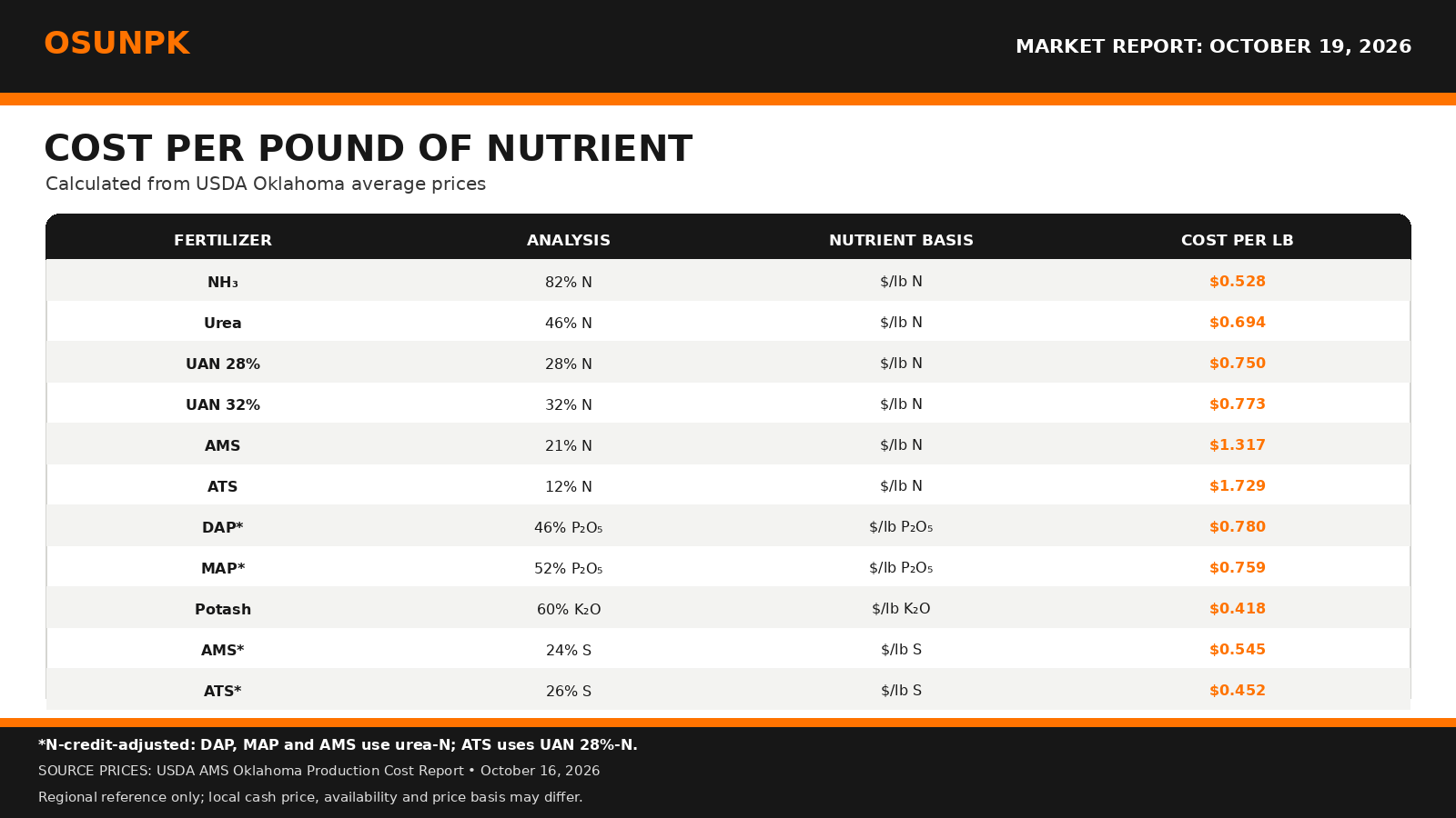
For Oklahoma producers and dealers, compare cash material quotes on the same pickup or FOB basis, use soil-test needs to guide nutrient purchases, and confirm availability before committing to an application plan. Fertilizer markets, local prices, and availability can change quickly and should be confirmed with local dealers.
Market Sources
- USDA Agricultural Marketing Service. Oklahoma Production Cost Report, October 16, 2026; retrieved October 19. https://www.ams.usda.gov/mnreports/ams_3621.pdf
- USDA Agricultural Marketing Service. Oklahoma Production Cost Report, September 18 and October 2, 2026. Preserved OSUNPK report observations used for changes; current-report endpoint: https://mymarketnews.ams.usda.gov/viewReport/3621
- Financial Express. “Import prices of urea down 60% since May peak,” October 18, 2026. https://www.financialexpress.com/policy/economy/import-prices-of-urea-down-60-since-may-peak/4364286/
- StoneX. “Phosphate Market Faces a Cost Floor That Demand Destruction Alone Cannot Break,” October 8, 2026. https://www.stonex.com/en/insights/phosphate-market-faces-a-cost-floor-that-demand-destruction-alone-cannot-break/
- Desmond, Tara. “What’s Really Driving Your Fertilizer Bill? StoneX’s Josh Linville Explains.” IL Corn, October 15, 2026. https://www.ilcorn.org/whats-really-driving-your-fertilizer-bill-stonexs-josh-linville-explains
- Two Rivers Cooperative. Fertilizer Index. Retrieval attempted October 19, 2026; table unavailable. https://www.tworiversks.coop/pages/custom.php?id=19995
This report is produced via Chat GPT Plus Work, with review by Brian Arnall.
Why is it difficult to find consistent effects of foliar fertilizers?
Understanding In-Season Nutrient Movement and Yield Impacts of Soybeans in the Southern Great Plains
Josh Lofton Cropping Systems Specialist.
Potassium can be a challenging nutrient to manage within a cropping system. Different rotations can highlight unique challenges that are exposed by environmental conditions such as drought or flooding. Throughout the year, the timing for adequate potassium can be very demanding.
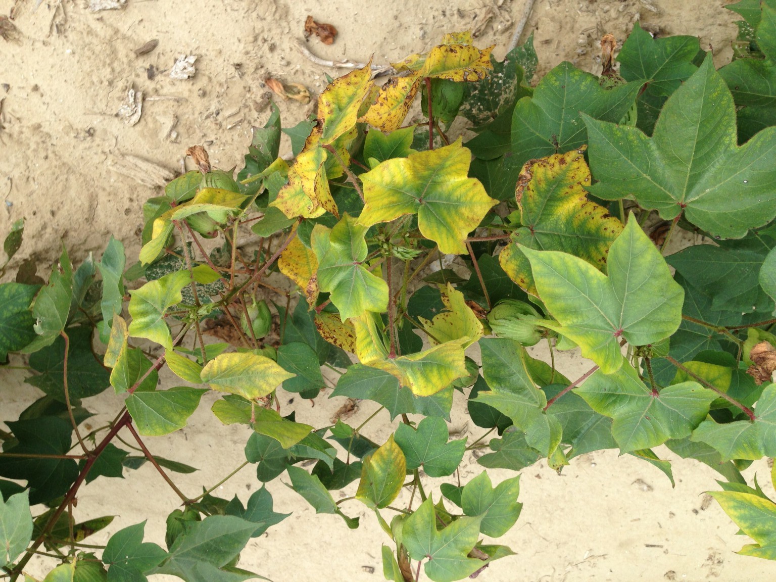
In recent years, there have been several instances of growers finding mid- to late-season potassium deficiencies that arise. These deficiencies still showed in soils that were not expected to have these issues based on soil tests. These mid-season potassium issues are typically in cotton and soybeans. However, in recent years, there have been growing number of fields of other crops as well as pastures seeing potassium issues. These issues have not typically or historically been present in these fields and pastures. This often leads to the question of, “Can foliar applications of potassium remedy issues this in-season?”
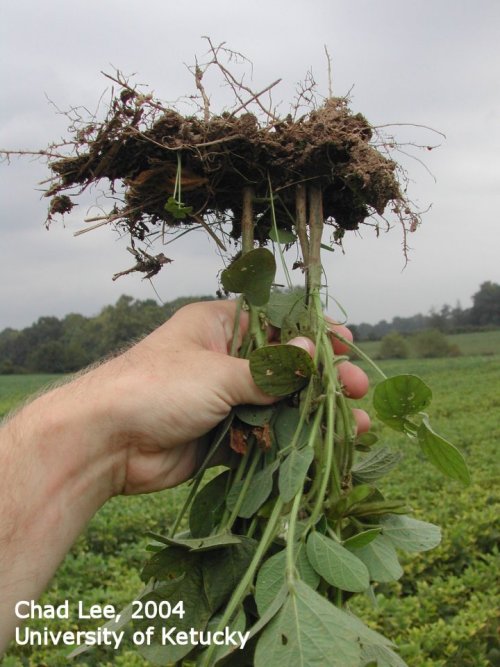
Foliar application of fertilizers is not a new concept. In fact, foliar fertilizers have been used for in-season micronutrient adjustments with some success. However, the physiological mechanisms between a macronutrient and micronutrients are quite different. I know reading this, many of you have been told by Brian Arnall himself that the difference between macronutrients (like potassium) and micronutrients (like copper and zinc, among others) is not importance, but the concentration that is needed within the plant.
This is where the issue with foliar application starts to arise. An important example is when speaking of macronutrients, we normally discuss concentration in terms of percent of total plant (grams of potassium per gram of plant material), whereas we discuss a micronutrient like zinc in ppm or parts per million (milligrams of zinc per kg of plant material). So, the scale of demand can differ widely between individual plants, and correcting a potassium deficiency may require applying several thousand-fold higher concentrations than a micronutrient.
Because of this, we wanted to track the concentration spike level of a foliar fertilization over a set time period following application to see how long the increased concentration was noted and if we could see it throughout the plant.
How the Study Was Conducted
A soybean trial was established in 2018 on a producer’s farm near Miami, Oklahoma, as well as the Mingo Valley Research Station near Bixby, Oklahoma. Data from these sites did not differ, so we combined the information into a single dataset. The study looked at a standard soil-applied fertilizer baseline (the control) compared against four different foliar potassium products applied at the R3 reproductive stage (beginning pod development):
- Soil applied only (Control)
- Soil applied + Potassium Thiosulfate
- Soil applied + Potassium Sulfate
- Soil applied + Potassium Hydroxide
- Soil applied + Potassium Thiosulfate and Potassium Acetate
For these, fertilizer was applied as a soil application of muriate of potash (0-0-60) at planting, based on soil test results. The control treatments recieved no additional applications of potassium beyond the initial soil applied. For the treatments, the different sources were then applied in addition to the fertilizer applied at planting.
To track exactly where the potassium moved after spraying, tissue samples were collected at 12, 24, 36, 48, 72, 120, and 192 hours after application. These samples were separated into leaves, petioles (leaf stems), and reproductive structures (flowers/pods/seeds). The samples were acid washed to remove any fertilizer residue on the surface of the leaves and analyzed for potassium content. Yield measurements were collected at the end of the season.
Did anything impact yields?
Of course, the first thing that needs to be addressed is yield. Results showed that there was not yield increase was seen across any treatment. This was not unexpected as most single applications of foliar fertilizers apply so few nutrients (not to mention the amount that is actually absorbed) that they often have little impact on total yield. These are often recommended to be applied multiple times over a period to provide enough nutrients to affect total concentration. It should be noted that total potassium concentration in the seeds, nor the protein or oil content was not impacted.
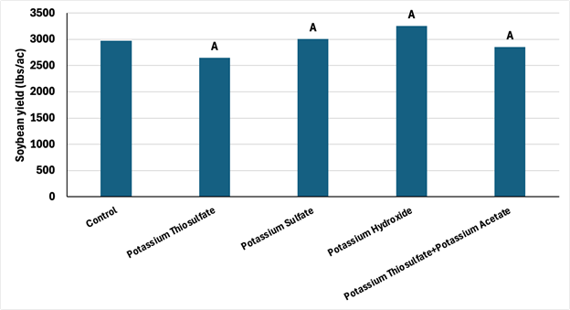
Figure 1. Impact of a single application of foliar fertilizer on soybean yields. Significances are shown by the lettering; different letters indicate significant differences between the individual treatments and the check. No comparison was made between the individual foliar treatments.
Impact of potassium concentration in the plant
All foliar fertilizers increased both leaf and petiole concentrations compared to treatments where fertilizer was only applied at planting. However, source does matter. Potassium thiosulfate alone or in with potassium acetate showed only a minor increase, reaching a 12% increase in leaf K at 36 hours and a 10% increase at 48 hours after application, respectively. From these levels, concentrations returned to levels near soil applied. The products composed of potassium hydroxide or sulfate, however, had an increase in leaf K of approximately 40% at 24 hours, which was held consistently through the 48-hour mark before returning to concentrations not different from the soil applied alone (at the 192-hour mark). This also translated to a similar increase in petiole concentration of 30% at 48-hours and held constant through the 72-hour mark before returning to concentrations not different than the soil applied alone.
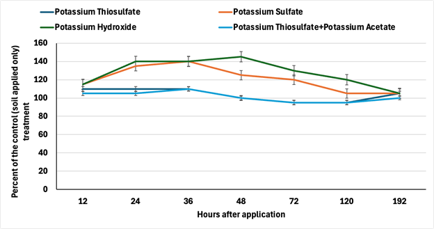
Figure 2. The impact of a single application of potassium foliar fertilizers on soybean leaf potassium concentration. The Y-axis indicates values compared to the control (soil applied only), where values under 100 indicate lower concentration and above 100 indicate an increased concentration.
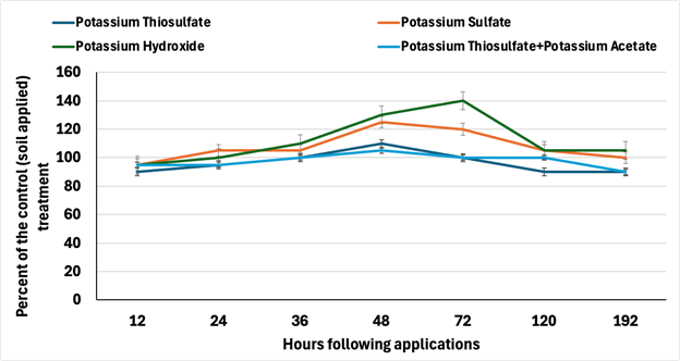
Figure 3. The impact of a single application of potassium foliar fertilizers on soybean petiole potassium concentration. The Y-axis indicates values compared to the control (soil applied only), where values under 100 indicate lower concentration and values above 100 indicate an increased concentration.
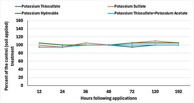
Figure 4. The impact of a single application of potassium foliar fertilizers on reproductive structures (flowers, pods, and seeds) and potassium concentration of the soybean plants. The Y-axis indicates values compared to the control (soil applied only) where values under 100 indicate lower concentration and above 100 indicate an increased concentration.
Several things impact this, but highlight that formulation, potassium source, and other components in the foliar applications matter. When looking at the concentration of the products, one is much different than the others. The potassium sulfate product has 30% potassium compared to the other that contain <20%. High concentration naturally results in a greater chance to have higher concentration inside the plant tissue (even if the percent of applied product is lower than other products). The other product that resulted in higher concentration within the plant was potassium hydroxide. This is a very soluble and small molecule that is easily taken up by the plant naturally.
Practical Takeaways for Producers and Consultants
- Temporary Fix, But Not Long-Term: Can these foliar applications make a difference in plant concentration? Yes, as shown by our data. However, this increased concentration was short-term and occurred almost entirely in the soybean leaf. Once the K moves into the petiole, the impact either decreased or was not present.
- Soil fertility basics are always better than recovery treatments: Foliar fertilizers are often considered a reactionary measure when deficiencies are found in the field. This isn’t always true, and these can be built into a fertility program; however, in many Oklahoma systems, environmental conditions are often the limiting factor compared to small concentration differences. Even if these would be yield limiting, they will often be covered/overshadowed by other factors. This leads me to the final take-home message…..
- Cost-Benefit Caution: A couple of factors came into this analysis. First and foremost, the raw data. Our data has shown no significant differences between the applied and non-applied treatments. This by itself makes seeing a consistent difference year in and year out, as well as in different systems, very unlikely. Second, as mentioned previously, several applications are often needed to make a significant difference on prolonged plant concentration.
While putting the final touches of this article, I was asked about the potential of these foliar fertilizers to improve bloom or pod retention even in the absence of major contributions to tissue concentration or yield. This one is a little tricky because there is some truth to the concept but can easily be taken out of context.
One potential deficiency of potassium deficiencies is early flower, pod, or even seed abortion. This can be due to various reasons. These can be due to reasons we normal assume, like drought. However, it can be for other more complex reasons like solute and source-sink dynamics. Since potassium plays such a critical role in loading (or pulling resources) into our reproductive structures, this can easily be seen.
Where things become a little nuanced is how impactful foliar fertilizers can be at overcoming these issues. These foliar applications do not have a hidden method for maintaining these reproductive structures but if a plant senses drought or lack of resources, it will adjust potential yield load to compensate.
An example of this is if the plant sense droughty conditions because you have low potassium and stomata regulation is not functioning as intended, yes a foliar fertilizer may address this need if it can overcome this deficiency. If we have a drought like the last couple of years, can foliar fertilizers be a way to overcome this, no. Stomata regulation is not the limiting factor, it is the lack of soil water.
This is why we cannot simply say yes/no on can this practice overcome an issues seen in-field. Because like most things in agricultural, in theory it is possible but there is nuanced to how it can happen.
Funding and support for this research were provided by the Oklahoma Soybean Board and the Oklahoma Agricultural Experiment Station.
OSUNPK Fertilizer Market Outlook: A Quiet Week Does Not Mean a Settled Market
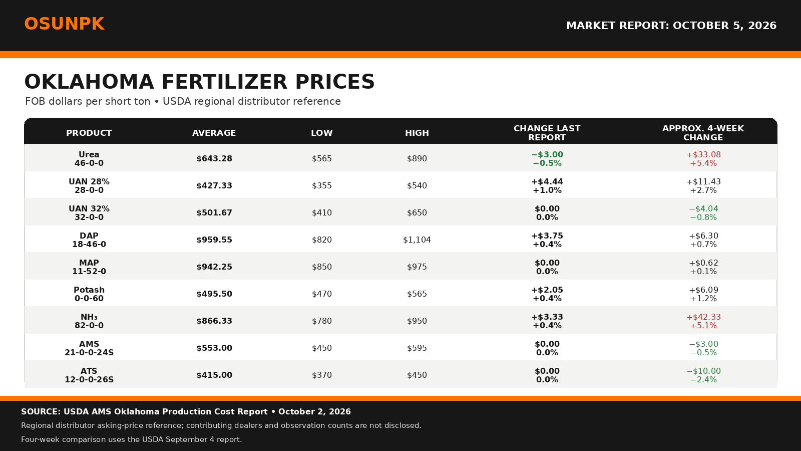
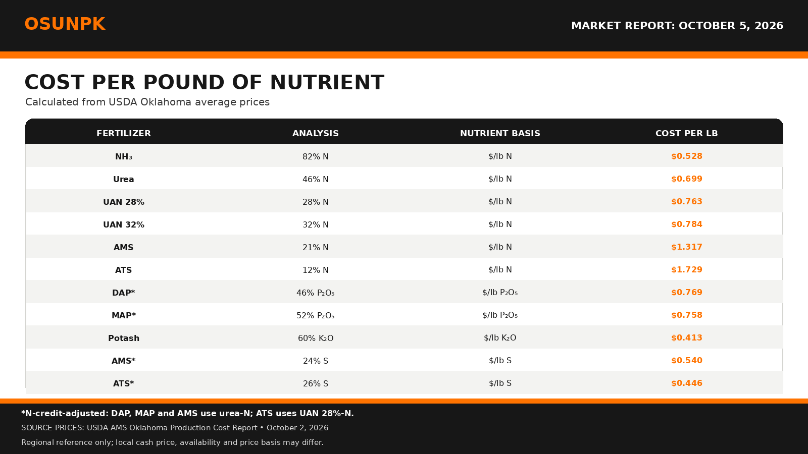
Oklahoma fertilizer prices were mostly a little higher in the October 2 USDA report, but the more important signal is what has happened over four weeks. Urea remains $33.08 per ton higher than September 4 despite easing $3.00 in the latest report, while anhydrous ammonia is up $42.33. The current report looks calm; the replacement-cost environment behind it is not.
Price-source note: The accompanying graphic’s Oklahoma average, minimum, and maximum come from the USDA Agricultural Marketing Service Oklahoma Production Cost Report. USDA does not identify contributing dealers. Named public dealer cash quotes, including Two Rivers Cooperative, are tracked separately and are not blended into USDA statistics.
Nitrogen markets continue to balance improving trade flows against persistent supply exposure. India has opened another tender for as much as 1.7 million metric tonnes of granular and prilled urea, with bids due October 7. A purchase of that size can redirect export tonnes and affect where other buyers, including Brazil and the United States, find supply. At the same time, international analysis indicates that urea and ammonia have retreated from their conflict-driven peaks, although seasonal demand could renew pressure while Persian Gulf shipping remains constrained.
Josh Linville’s latest public commentary focuses on the structural side of that risk. He argues that the United States remains exposed because imported nitrogen is vulnerable to overseas production problems and logistics disruptions. That does not mean every disruption produces an immediate Oklahoma price increase, but it helps explain why local values can remain firm even when an international benchmark softens. Urea’s mixed movement in the current USDA report is consistent with dealers carrying inventory purchased at different replacement costs.
Phosphate deserves attention even though Oklahoma DAP and MAP changed very little. Sulfur shortages remain a constraint on phosphate production, and uncertainty continues around Chinese DAP and MAP exports. Linville has also noted that temporary duty relief on Moroccan phosphate has not translated quickly into lower U.S. farm prices because the global market remains tight. Higher ammonia and sulfur costs can support DAP and MAP before that pressure becomes obvious in a local price series. AMS and ATS were unchanged this period, but sulfur availability still connects those products to the broader phosphate cost structure.
Potash remains comparatively well supplied. Discussion of possible U.S. purchases from Belarus attracted attention, but Linville told Reuters that additional Belarusian supply would probably have limited effect because the United States is not currently struggling to source potash. Freight and trade policy still matter, but nitrogen and phosphate carry the larger near-term supply risks.
Over the next two weeks, watch India’s tender results, Brazilian urea demand, fall NH₃ movement, sulfur availability, phosphate operating rates, and whether Oklahoma urea contacts begin moving in the same direction. The present mix argues for monitoring rather than a confident price forecast.
For Oklahoma producers and dealers, compare cash quotes on the same pickup or FOB basis and separate material price from application and delivery. The wide local urea range makes dealer-specific confirmation especially important before committing to product.
Fertilizer markets, local prices, and availability can change quickly. Confirm current prices and terms with local dealers before purchasing.
Market Sources
- USDA Agricultural Marketing Service. Oklahoma Production Cost Report, October 2, 2026. https://www.ams.usda.gov/mnreports/ams_3621.pdf
- Indian Potash Limited. Tender Notice IPL/UREA/2026-27/02, September 23, 2026. https://indianpotash.org/tender.html
- Glauber, Joseph, and Shawn Arita. “How are fertilizer markets coping with the continued closure of the Strait of Hormuz?” IFPRI/CGIAR, September 18, 2026. https://www.cgiar.org/news-events/news/how-are-fertilizer-markets-coping-continued-closure-strait-hormuz
- Linville, Josh. “America’s Nitrogen Import Habit Leaves Farms Exposed to Supply Shocks.” StoneX, September 29, 2026. https://www.stonex.com/en/insights/america-s-nitrogen-import-habit-leaves-farms-exposed-to-supply-shocks/
- Reuters. “Trump says US is working on deal to purchase potash from Belarus,” September 21, 2026. https://www.reuters.com/world/americas/trump-says-us-is-working-deal-purchase-potash-belarus-2026-09-21/
- S&P Global Commodity Insights. “China DAP, MAP exports remain uncertain as September begins,” September 2, 2026. https://www.spglobal.com/energy/en/news-research/latest-news/agriculture/090226-china-dap-map-exports-remain-uncertain-as-september-begins
This report is produced via Chat GPT Plus Work, with review by Brian Arnall.
OSUNPK Fertilizer Market Outlook: Urea Turns Higher in an Uneven Market
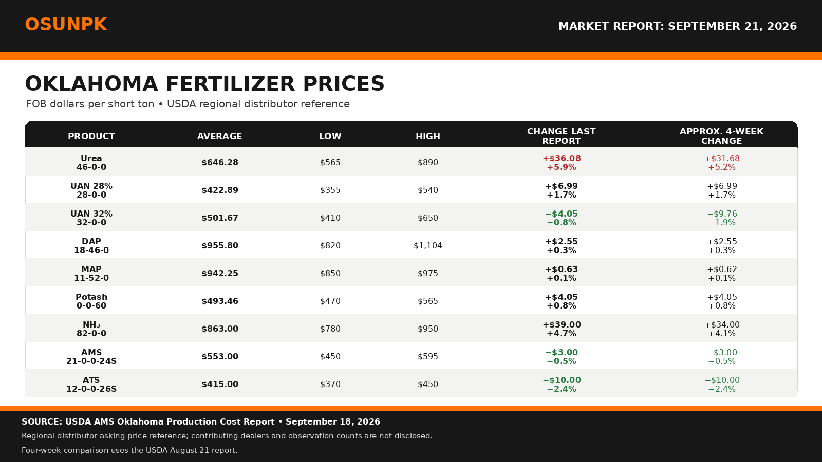
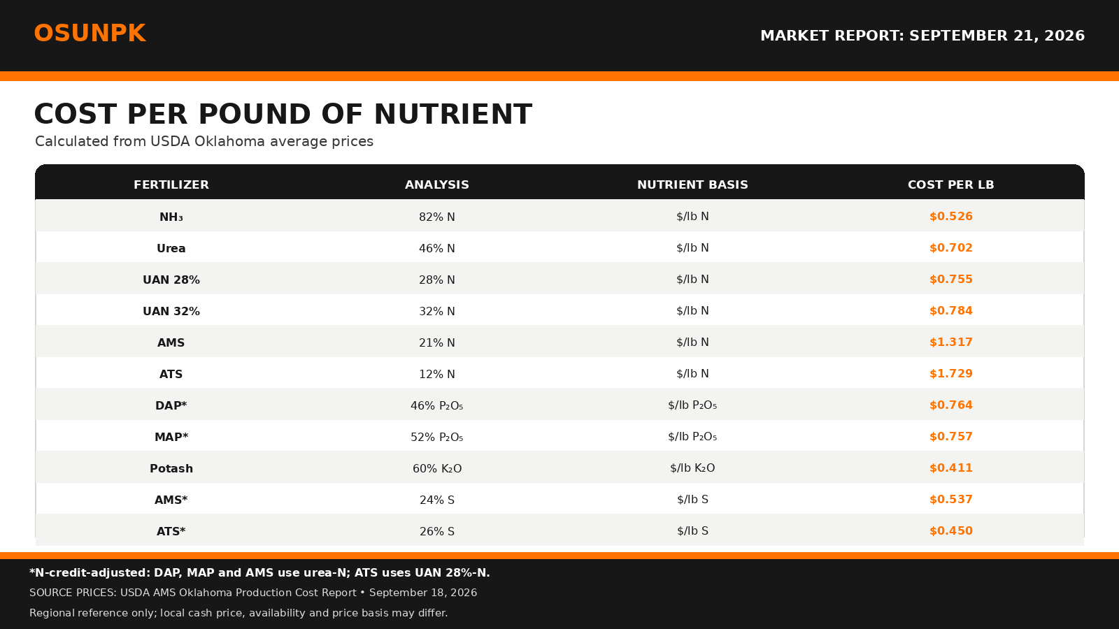
Oklahoma’s clearest fertilizer move over the past two weeks was urea’s return to higher ground. The September 18 USDA average rose $36.08 per ton, or 5.9%, to $646.28. Anhydrous ammonia also increased $39 per ton, while UAN 28% edged higher and UAN 32% slipped. The split among nitrogen products is a useful reminder that one product’s direction does not automatically describe the whole nitrogen market.
Price-source note: The accompanying graphic’s Oklahoma average, minimum, and maximum come from the USDA Agricultural Marketing Service Oklahoma Production Cost Report. USDA does not identify contributing dealers. Named public dealer cash quotes, including Two Rivers Cooperative, are tracked separately and are not blended into USDA statistics.
USDA described urea as the clear exception in an otherwise uneven market, with increases reported consistently across its contacts. That local move contrasts with recent evidence of softer international urea values. India’s landed import cost reportedly fell to about $406 per metric tonne in August, 57% below its May peak, while Indian stocks reached 7.51 million tonnes—78% above a year earlier. Those numbers suggest improved global availability, but they do not guarantee lower Oklahoma replacement costs. Timing, inland freight, dealer inventory position, product form, and the price paid for the next load can create a different local signal.
Anhydrous ammonia’s increase deserves attention as fall application approaches, even though it remained below its July level. UAN’s mixed movement also fits a market in which inventory coverage differs by product. In August, fertilizer analyst Josh Linville noted that UAN and ammonia manufacturers had strong forward sales positions even as urea benchmarks weakened. That observation remains relevant to the current divergence, though it should be treated as market context rather than a forecast.
Phosphate prices barely moved in the Oklahoma report, but the cost picture underneath them is less quiet. USDA said phosphorus-fertilizer production inputs have risen sharply, adding upward pressure and near-term uncertainty. International reporting also placed August DAP values above April levels, with freight disruptions cited as a factor. Ammonia and sulfur are major variable inputs in phosphate production, so strength or supply disruption in either market can eventually affect DAP and MAP replacement values. AMS and ATS moved lower locally this period, but sulfur-market risk remains relevant to both products and to phosphate manufacturing.
Another cost pressure sits outside the fertilizer table. USDA reported Oklahoma farm diesel up $0.72 per gallon in two weeks to a record $5.44 average for this series. The fertilizer graphics exclude delivery and application charges, as they should, but higher fuel costs can still raise the total cost of getting product to the field.
Over the next several weeks, watch whether Oklahoma urea gains persist across another report, whether fall NH₃ demand strengthens, and whether phosphate input pressure reaches posted retail values. India’s purchasing pace, global urea availability, sulfur and ammonia supply, freight, and local moisture conditions all remain important. These forces are pulling in different directions, so the present data support caution rather than a definitive price call.
For Oklahoma producers and dealers, compare products on both a cash-per-ton and nutrient-cost basis, then verify pickup or FOB terms and all service charges. Where soil tests allow flexibility, product fit, timing, and availability may matter as much as the posted price.
Fertilizer markets, local prices, and availability can change quickly. Confirm current prices and terms with local dealers before purchasing.
Market Sources
- USDA Agricultural Marketing Service. Oklahoma Production Cost Report, September 18, 2026. https://www.ams.usda.gov/mnreports/ams_3621.pdf
- Financial Express. “Import prices of urea down 57% since May peak,” September 15, 2026. https://www.financialexpress.com/policy/economy/import-prices-of-urea-down-57-since-may-peak/4339998/
- Hoosier Ag Today. “Fertilizer Markets at a Crossroads: StoneX’s Josh Linville Reveals the Biggest Risks—and Where Growers Should Buy Now,” August 12, 2026. https://www.hoosieragtoday.com/2026/08/12/josh-linville-fertilizer-markets/
- CoBank. “Why higher fertilizer prices are here to stay,” August 13, 2026. https://www.cobank.com/knowledge-exchange/why-higher-fertilizer
This report is produced via Chat GPT Plus Work, with review by Brian Arnall.
Soil Your Undies: When a Great Demo Gets Asked to Do Too Much
I often say that in K–12 education we teach a lot of things in black and white. Students first need to understand the basic concepts: plants need nutrients, microorganisms decompose organic matter, and soils are biologically active. Then somewhere through a bachelor’s degree, or simply through enough years of experience, we learn that agriculture is rarely that black and white. There are a lot of shades of gray. Keep studying, researching, farming, or advising long enough and you eventually realize there aren’t just 256 shades of gray. There is also ROYGBIV. There is a whole spectrum of interactions and conditions that determine what happens in the soil.
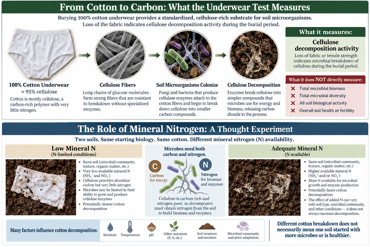
I think the “Soil Your Undies” demonstration fits that progression perfectly. It is a great black and white teaching tool. Bury a pair of 100% cotton underwear, wait several weeks, and dig them back up. Sometimes there isn’t much left besides the elastic waistband. Students can see that something happened belowground, and that opens the door to conversations about microorganisms, decomposition, carbon cycling, and the fact that soil is a living system. As a teaching demonstration, that is hard to beat.
Where I become more cautious is when we take that intentionally simple lesson and make a much more complicated conclusion: the pair with less cotton remaining came from the healthier soil or represents the better management practice. That is where we need to move beyond black and white.

To begin with we must know what the microbes are eating.
Cotton fiber itself gives us the first clue about what this test measures. Cotton is approximately 95% cellulose, and standardized cotton strips have been used by soil scientists for decades specifically as an index of cellulose decomposition (Latter et al., 1988; Tiegs et al., 2013). Cellulose is a long chain of glucose molecules and one of the major structural components of plant material. Its decomposition depends on organisms capable of producing cellulolytic enzymes that break those chains into smaller compounds that microorganisms can use.
Therefore, when cotton underwear disappears, we can make a scientifically defensible statement: the soil environment supported cellulose decomposition during the time the underwear was buried. That is useful information but notice how specific that statement is. We did not measure the total number of microorganisms, microbial diversity, or every biological process occurring in that soil, and we certainly did not measure everything encompassed by the much broader term soil health. Research comparing cotton-strip decomposition with microbial biomass illustrates that distinction. Walton and Allsopp (2007) found a relatively poor relationship between cotton-strip measurements and microbial biomass measured by substrate-induced respiration (r² = 0.26). They recommended using cotton strips alongside other physical and chemical soil indicators rather than as a stand-alone biological measurement. Soil can contain a substantial microbial population without necessarily destroying a pair of underwear quickly.
Is breaking down cellulose what the soil needs to be doing?
Cellulose decomposition is important. Crop residues contain cellulose, and their decomposition is part of carbon and nutrient cycling. But agriculture does not necessarily need every microbial process operating at its maximum rate all the time. Depending on the production system, time of year, and management objective, we may be more interested in nutrient mineralization or immobilization, aggregate formation, disease suppression, nitrogen transformations, carbon stabilization, or simply keeping residue on the soil surface. Faster cellulose decomposition is therefore not automatically better; it tells us that this specific biological process was occurring more rapidly under those conditions. This does not make the cotton test wrong. It means we need to be precise about the question it answers.
The scientific cotton-strip assay has successfully detected differences in cellulose decomposition among soils and management systems. Nachimuthu et al. (2022), for example, found differences in cotton-strip degradation among long-term crop rotation and tillage treatments. That supports the conclusion that management can affect cellulose decomposition. It does not automatically establish that the management practice producing the fastest cellulose decomposition created the healthiest soil. Margenot and Wade (2023) raised a similar concern about the interpretation of soil enzyme activities, cautioning against taking a measurement of a specific biological process and assuming that it scales directly to broader soil functions or outcomes. Measuring a process and determining what that process means for the functioning of the soil are two different questions.
Now add some gray: nitrogen
This is where the soil fertility specialist in me starts asking questions. Cotton provides microorganisms with a lot of carbon but almost no nitrogen. Yet microorganisms cannot live on carbon alone. They need nitrogen to produce proteins and enzymes and to build new microbial biomass. The microorganisms colonizing that cotton therefore must obtain much of what they need from the surrounding soil. Imagine taking one soil and thoroughly mixing it. We start with the same microbial community, organic matter, texture, pH, temperature, and water content. Divide it into two treatments and bury identical pieces of cotton. The only major difference is mineral nitrogen: one treatment has very little available NH₄-N and NO₃-N, while the other has an adequate supply. Would the underwear necessarily decompose at the same rate? There is good reason to believe it may not.
Nottingham et al. (2018) examined nutrient limitation during cellulose decomposition by adding cellulose and individual nutrients to soils. Nitrogen addition produced the largest fungal growth response associated with cellulose, and the researchers concluded that nitrogen was an important limitation to fungal growth and cellulose decomposition in the soils they studied. The implication for our underwear is important. Cotton in the higher N soil could potentially disappear faster without that soil starting with more microorganisms or a “healthier” microbial community. The organisms capable of decomposing cellulose may simply have better access to the nitrogen required to grow and produce the enzymes needed to exploit this large carbon source. That does not mean adding nitrogen fertilizer will always make underwear disappear faster. Microbial responses to N depend on the soil, microbial community, nutrient status, substrate, and environment. Other nutrients may become limiting, and long-term N additions can alter microbial communities and decomposition processes in ways that are very different from a short-term response to available N. That complexity is exactly the point: we started with a black-and-white demonstration of biological activity, but bringing in the mineral N conversation now add many shades of gray.
Then comes pH—and more color
Soil pH adds another layer because it does more than simply make microbes “more” or “less” active. It can change which groups of microorganisms are most active. I have plenty of work discussing how quickly soil pH can change across landscape and how much our management also significantly impacts soil pH. Across agricultural soils, bacterial growth and diversity generally increase as strongly acidic soils approach neutral conditions, while fungi tend to become relatively more important as pH declines. Rousk et al. (2009, 2010), working across soils ranging from approximately pH 4 to 8, documented substantial shifts in bacterial and fungal growth and in the fungal relationship across the pH gradient. That distinction matters for an underwear test because both bacteria and fungi participate in cellulose decomposition. A lower-pH soil may have reduced bacterial growth while maintaining a comparatively greater fungal contribution. At a higher pH, the balance can shift toward bacteria. The microbial community doing the work can therefore change substantially without a corresponding black-and-white change from “poor biology” to “good biology.”
There is also evidence that pH can affect cellulose decomposition itself. Work with volcanic soils found that cellulose decomposition potential was related to both soil pH and microbial N availability, rather than simply to the amount of microbial biomass present. This creates an interesting possibility for the underwear demonstration: two soils could contain similar amounts of microbial biomass but decompose cotton at different rates because one provides a more favorable chemical and nutritional environment for the organisms capable of using cellulose. I would also be careful about turning that into another simple rule such as “higher pH equals faster cotton decomposition.” As soils move from strongly acidic conditions toward the range where many agricultural crops are grown, bacterial activity generally increases, but fungi, bacteria, extracellular enzymes, nutrient availability, and cellulose decomposition do not all respond to pH in exactly the same way. Very acidic conditions can suppress some processes while favoring organisms better adapted to acidity. That is a much more interesting biological story than simply labeling one soil as having more microbial activity than another.
Then comes ROYGBIV
Nitrogen and pH are only two variables. Soil moisture determines whether microorganisms can remain active and whether substrates and nutrients can move through the soil. Texture influences water retention, aeration, nutrient availability, aggregation, and microbial habitat, so identical cotton buried in a sandy soil and a clay soil is not necessarily experiencing the same environment. Phosphorus, sulfur, or another nutrient can limit microbial growth even when carbon and nitrogen are abundant. Finally, the microbial community itself matters because different bacterial and fungal populations differ in their ability to produce the enzymes needed to attack cellulose.
What we see when we dig up the underwear is therefore the integrated result of microbial community × substrate × nitrogen × other nutrients × moisture × pH × texture × time, along with interactions among them. A difference in cotton decomposition is real, but the underwear alone cannot tell us which of those factors produced the difference. More importantly, it cannot tell us whether the difference represents better or worse management. That distinction between a soil health indicator and the soil function or outcome it is intended to represent is increasingly being emphasized in the soil health literature (Maharjan et al., 2024).
That is no longer black and white. That is ROYGBIV.
Keep burying the underwear
None of this is an argument to stop Soil Your Undies. Keep doing it. Use it in classrooms, bury underwear at field days, have students predict what will happen, and put underwear in contrasting soils so they can see that decomposition happens below ground. It makes an invisible biological process visible, and that makes it a great teaching tool.
Where I think we need to be more careful is when we turning that demonstration into a scorecard for soil health or management practices. A producer should not dig up two pairs of underwear and conclude that the field with less cotton remaining necessarily has more microorganisms, better management, greater fertility, or healthier soil. Too many biological, chemical, and environmental factors influence cellulose decomposition for the underwear alone to support those conclusions.
Perhaps that distinction provides an even better way to use the demonstration. With younger students, Soil Your Undies can teach the black and white: microorganisms live in soil and decompose organic materials. With more advanced students, farmers and agronomists, the same demonstration can teach the gray by asking, why did these two pieces of cotton decompose differently? Once we start asking about water, nitrogen, pH, texture, nutrients, microbial communities, and all of the possible interactions, we get to ROYGBIV.
This distinction becomes especially important when the demonstration is used with students or audiences without an agricultural or soil science background. If two management systems are compared and the one with less cotton remaining is presented as the “better” practice, we may be teaching a conclusion the test cannot support. Those audiences may not yet have the background to recognize the effects of moisture, nitrogen, pH, texture, or microbial community on cellulose decomposition. The demonstration can then unintentionally introduce bias toward management practice rather than teach how complex soil biological processes really are.
So, keep burying the underwear. Just don’t ask it to answer more than it can.
References
- Chew, I., Obbard, J.P., & Stanforth, R.R. 2001. Microbial cellulose decomposition in soils from a rifle range contaminated with heavy metals. Environmental Pollution 111:367–375. doi:10.1016/S0269-7491(00)00094-4.
- Latter, P.M., Bancroft, G., & Gillespie, J. 1988. Technical aspects of the cotton strip assay in soils. International Biodeterioration 24:25–47. doi:10.1016/0265-3036(88)90073-5.
- Maharjan, B., Das, S., Thapa, V.R., & Sharma Acharya, B. 2024. Soil health cycle. Agrosystems, Geosciences & Environment 7:e20504. doi:10.1002/agg2.20504.
- Margenot, A.J., & Wade, J. 2023. Getting the basics right on soil enzyme activities: A comment on Sainju et al. (2022). Agrosystems, Geosciences & Environment 6:e20405. doi:10.1002/agg2.20405.
- Nachimuthu, G., Hundt, A., Palmer, B., Schwenke, G.D., & Knox, O.G.G. 2022. Cotton strip assay detects soil microbial degradation differences among crop rotation and tillage experiments on Vertisols. Journal of Microbiological Methods 200:106558. doi:10.1016/j.mimet.2022.106558.
- Nottingham, A.T., Hicks, L.C., Ccahuana, A.J.Q., Salinas, N., Bååth, E., & Meir, P. 2018. Nutrient limitations to bacterial and fungal growth during cellulose decomposition in tropical forest soils. Biology and Fertility of Soils 54:219–228. doi:10.1007/s00374-017-1247-4.
- Rousk, J., Brookes, P.C., & Bååth, E. 2009. Contrasting soil pH effects on fungal and bacterial growth suggest functional redundancy in carbon mineralization. Applied and Environmental Microbiology 75:1589–1596.
- Rousk, J., Bååth, E., Brookes, P.C., Lauber, C.L., Lozupone, C., Caporaso, J.G., Knight, R., & Fierer, N. 2010. Soil bacterial and fungal communities across a pH gradient in an arable soil. ISME Journal 4:1340–1351.
- Tiegs, S.D., Clapcott, J.E., Griffiths, N.A., & Boulton, A.J. 2013. A standardized cotton-strip assay for measuring organic-matter decomposition in streams. Ecological Indicators 32:131–139. doi:10.1016/j.ecolind.2013.03.013.
- Walton, N.G., & Allsopp, D. 2007. Comparison of methods for measuring soil microbial activity using cotton strips and a respirometer. Journal of Microbiological Methods 69:322–329.
OSUNPK Fertilizer Market Outlook: Nitrogen Decline Pauses 9.7.26
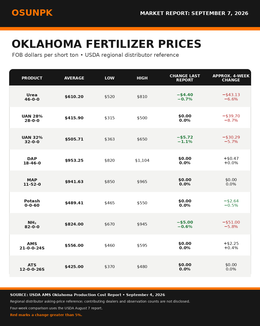
The most important fertilizer-market development of the past two weeks is not another sharp price move, but the pause that followed August’s nitrogen decline. Oklahoma’s September 4 report shows urea down only $4.40 per ton, UAN 32% down $5.72, and anhydrous ammonia down $5.00. UAN 28%, phosphate, potash, AMS, and ATS were unchanged. Looking back four weeks, however, the nitrogen correction remains substantial: urea is down 6.6%, UAN 28% is down 8.7%, UAN 32% is down 5.7%, and NH3 is down 5.8%.
Price-source note: The accompanying graphic’s Oklahoma average, minimum, and maximum come from the USDA Agricultural Marketing Service Oklahoma Production Cost Report. USDA does not identify contributing dealers. Named public dealer cash quotes, including Two Rivers Cooperative, are tracked separately and are not blended into USDA statistics.
USDA attributes the quiet local market to weak demand under persistent heat and drought. That distinction matters. Stable prices caused by limited field activity do not necessarily indicate that replacement costs or global supply risks have settled. As fall demand develops, local bids may respond differently depending on dealer inventory, transportation, and when replacement tons were purchased.
Nitrogen markets continue to balance large international buying programs against improved availability. In recent public commentary, StoneX fertilizer analyst Josh Linville pointed to India’s 1.7-million-ton urea purchase and identified Brazil as the next major demand cycle to watch. A completed Indian tender can absorb prompt supply, but the next direction depends on whether Brazilian demand arrives strongly enough to keep exporters engaged. Product type also matters because Brazil typically needs granular urea, while much of China’s available export supply has been prilled.
Phosphate remains a different story. Oklahoma DAP and MAP prices were unchanged, but the global market still carries support from restricted Chinese exports and elevated sulfur and ammonia costs. Linville also highlighted the arrival of Moroccan phosphate cargoes following the suspension of U.S. countervailing duties, including an MAP vessel that is more relevant to U.S. demand than the earlier TSP shipment. Additional import competition could improve availability, but one or two vessels do not by themselves reset the market.
Sulfur is part of that phosphate equation. It is required to manufacture phosphoric acid, so constrained sulfur trade can support DAP and MAP production costs. The same global pressure does not translate directly into identical local movement for AMS and ATS; both remained unchanged in Oklahoma this period. Those products should therefore be evaluated on actual sulfur need, formulation, and local cash price rather than assumed movement from phosphate headlines.
The next items to watch are Oklahoma rainfall and fall field activity, Brazilian urea purchasing, additional Indian tenders, Chinese export volumes, Moroccan phosphate arrivals, sulfur availability, and inland freight. These forces remain capable of moving in opposite directions, so the current pause should not be read as a firm price forecast.
For Oklahoma producers, this is a good time to compare products on both dollars per ton and cost per pound of the needed nutrient. Quotes should be placed on the same pickup or FOB basis, with application, blending, delivery, and tax separated before making comparisons.
Fertilizer markets, local prices, and availability can change quickly. Confirm current prices and terms with local dealers before purchasing.
Market Sources
- USDA Agricultural Marketing Service. Oklahoma Production Cost Report, September 4, 2026. https://www.ams.usda.gov/mnreports/ams_3621.pdf
- Josh Linville, StoneX. Public fertilizer-market commentary on India’s urea tender, Brazil’s demand cycle, and Moroccan phosphate arrivals. https://www.linkedin.com/posts/joshua-linville-9555a711_indias-urea-tender-just-gave-a-fading-rally-activity-7488273113961476098-Mepg
- CoBank. Why Higher Fertilizer Prices Are Here to Stay, August 13, 2026. https://www.cobank.com/knowledge-exchange/why-higher-fertilizer-prices-are-here-to-stay
- World Trade Organization. Fertilizer Trade Impacted by Strait of Hormuz Conflict, July 10, 2026. https://www.wto.org/english/blogs_e/data_blog_e/blog_dta_10jul26_451_e.htm
This report is produced via Chat GPT Plus Work, with review by Brian Arnall.
2026 Grain Sorghum Variety Trial Results: Tipton and Chickasha
Josh Lofton Cropping System Specialist, OSU
Tipton:
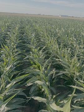
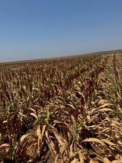
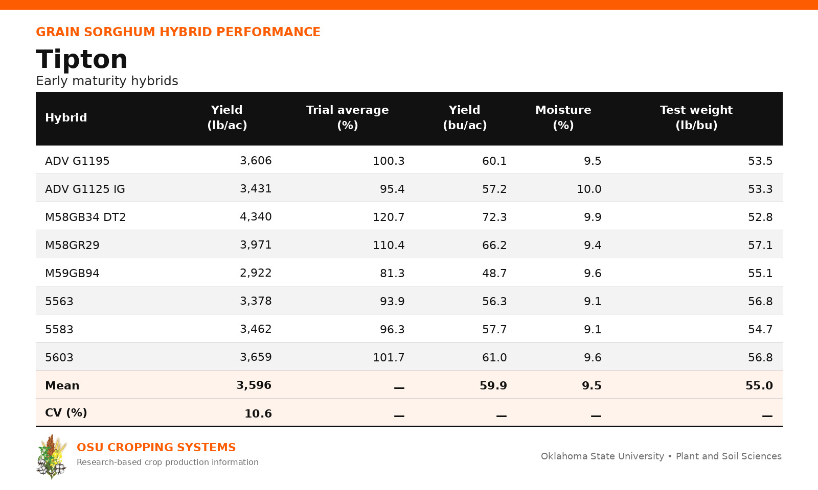
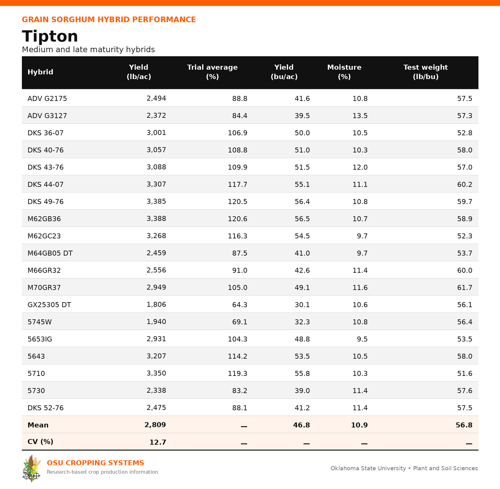
The southern most location in our sorghum plots is often the first to be planted and the first to be harvested. However, in the last couple of years, moisture has resulted in having to wait for appropriate moisture to be present to successfully establish the crop. This year, the plots were planted on April 21st and harvested on August 13th. As with all of our dryland plots, we seeded the plots to approximately 45,000 seeds/ac with the hope of getting stands, at minimum, between 30,000 to 35,000 plants/ac. This was located on the Oklahoma State University research station just south of Tipton Oklahoma. Overall, minimal pressure was noted throughout the year. This is unique for this location, being close to Texas and located where it is on station, pest and late-season bird pressure is common. Weeds were maintained mainly through the use of preplant herbicide program (labeled rates of S-Metolachlor and Atrazine). Outside of the yield, moisture and test weight values in the graph, averages for each column are provided as well as CV for the trial. This CV value is a measure of the variability between the individual varieties throughout the trial. A CV value below 15% is considered very good with most differences in average yields being associated with performance and not environmental, soil, or management differences.
Chickasha:
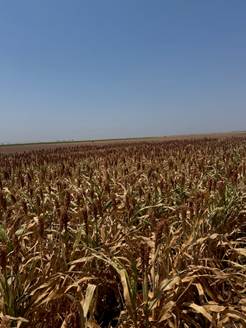
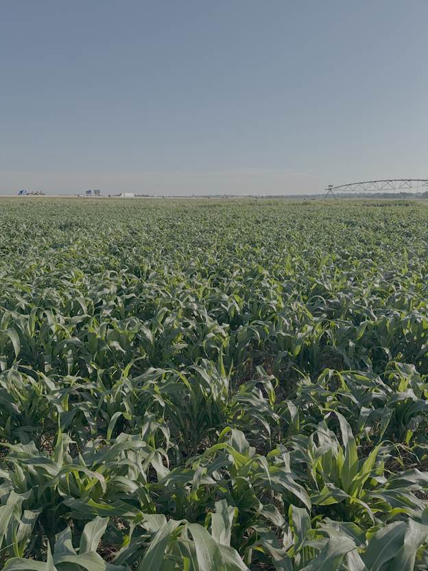
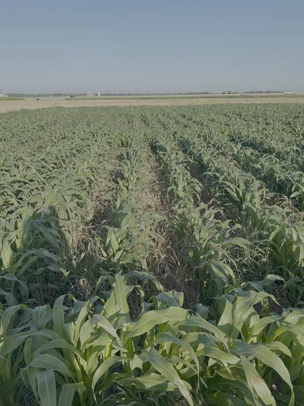
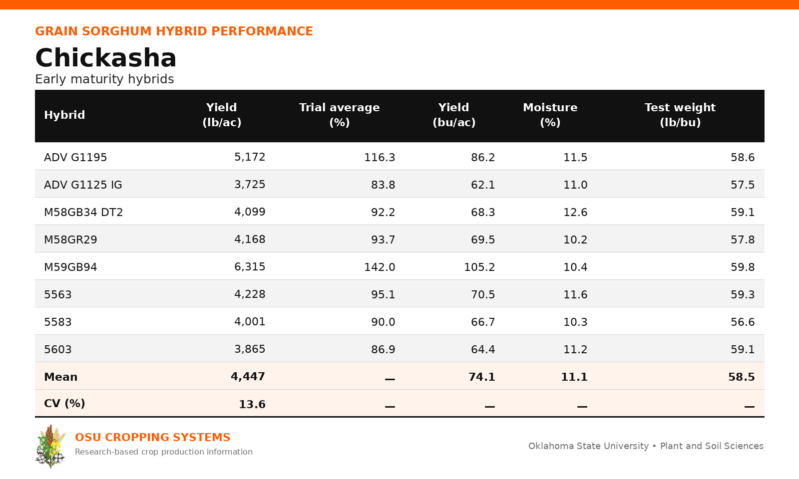
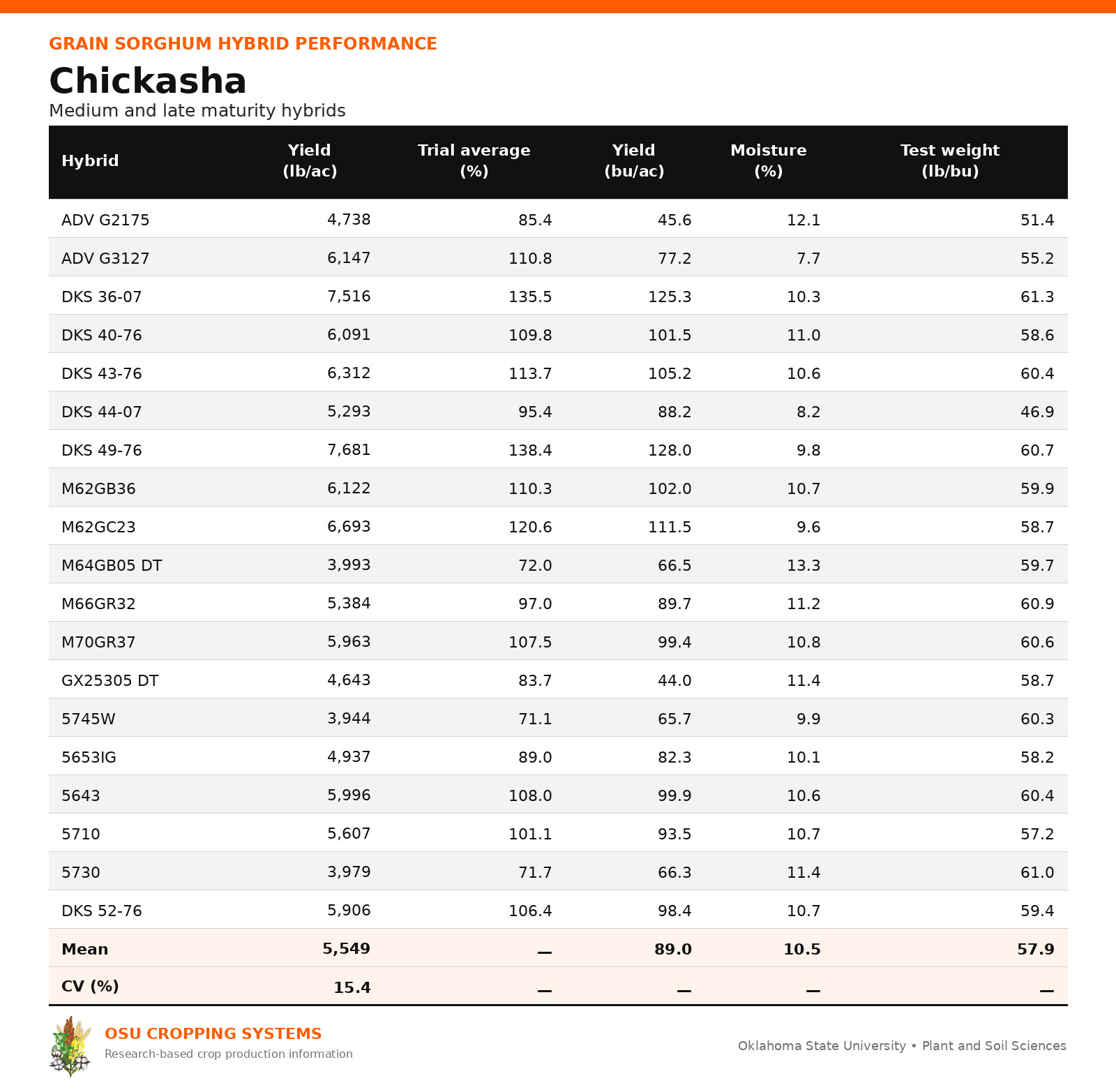
Our Chickasha location was planted a little later than intended; however, the crop went into a terminated wheat stand and had to work with periods of wet conditions in late April that pushed planting into early May. Harvest occurred in late August (the 20th) after a glyphosate desiccation treatment. As with all of our dryland plots, we seeded the plots to approximately 45,000 seeds/ac with the hope of getting stands, at minimum, between 30,000 to 35,000 plants/ac. This trial was located at the Oklahoma Research and Extension Center outside of Chickasha, Oklahoma. There was minor pest pressure throughout the season, with grasshopper, sorghum aphids, and chinch bugs being present but not to levels that require any management. The aphids and chinch bugs were only present during the latest part of the season during grain dry down. Weeds were the primary issues with this location this season. While most years have a prominent johnsongrass and pigweed issue, crabgrass was primary issue this season. Impact was minimized by manually weeding the plots several times throughout the season. Outside of the yield, moisture and test weight values in the graph, averages for each column are provided as well as CV for the trial. This CV value is a measure of the variability between the individual varieties throughout the trial. A CV value below 15% is considered very good with most differences in average yields being associated with performance and not environmental, soil, or management differences.
For any questions please contact Josh Lofton at josh.lofton@okstate.edu
OSUNPK Fertilizer Market Outlook: Local Nitrogen Prices Break Lower 8.24.26
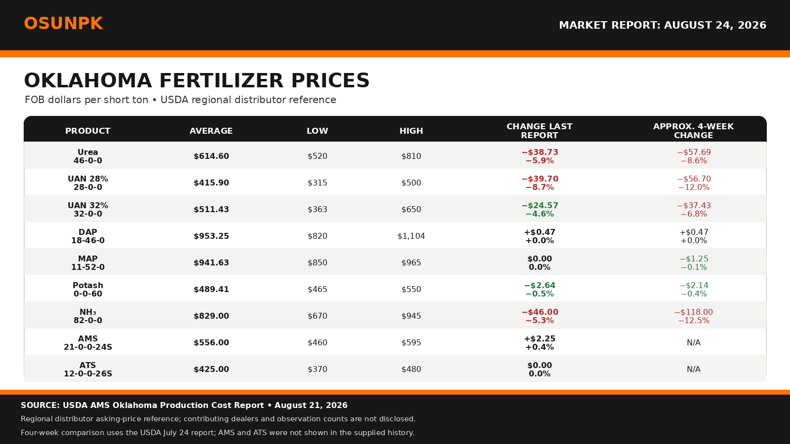
The most important movement of the past two weeks is the decline in Oklahoma nitrogen references. From August 7 to August 21, UAN 28% fell $39.70 per ton, urea fell $38.73, and anhydrous ammonia fell $46.00. USDA attributes the weakness to reduced demand as persistent heat and limited rainfall constrain field activity across the state.
Price-source note: The accompanying graphic’s Oklahoma average, minimum, and maximum come from the USDA Agricultural Marketing Service Oklahoma Production Cost Report. USDA does not identify its contributing dealers. Named public dealer cash quotes, including Two Rivers Cooperative, are monitored separately and are not blended into the USDA statistics.
The local decline does not mean that global nitrogen risk has disappeared. StoneX reported August 19 that India secured about 1.7 million metric tons in its latest urea tender with ample offers, including an expected contribution from China. That supply response eased immediate pressure, but attention now shifts toward Brazil’s September-through-December import window. Brazil needs granular urea, while much of China’s available export supply is prilled, so timing, product form, and destination still matter.
Josh Linville’s August 12 market commentary likewise described a well-supplied Indian tender and a weaker NOLA urea market, while cautioning that UAN and ammonia manufacturers held strong forward sales books. That distinction matters in Oklahoma: a softer urea benchmark can move faster than UAN or ammonia when producers have already covered substantial forward demand. Local weather can amplify the difference by weakening spot demand even while manufacturer positions remain supported.
Phosphate prices were nearly unchanged in the Oklahoma report, but their cost structure remains exposed to ammonia and sulfur. CoBank noted August 13 that Middle East disruptions and Russian supply constraints have affected ammonia production and sulfur availability, while China’s phosphate exports remain sharply restricted. Linville also highlighted sulfur as a bottleneck because a large share of globally traded sulfur normally moves through the Strait of Hormuz. Those pressures can raise the cost of producing DAP and MAP even when local posted values are temporarily steady. They also deserve attention for AMS and ATS, although Oklahoma’s reported averages changed little this period.
Potash remains the quietest major nutrient. Its production base is less directly tied to Middle East natural gas and sulfur, although ocean freight and broader logistics can still affect delivered replacement costs.
Over the next several weeks, watch Oklahoma rainfall and fall field demand, Brazil’s urea buying pace, the mix of Chinese exports, further Indian tenders, phosphate operating rates, sulfur availability, and freight. These forces point in different directions, so the current local nitrogen decline should be read as a market development rather than a definitive forecast.
For Oklahoma producers and dealers, the practical step is to compare current cash quotes on the same pickup or FOB basis and separate material price from delivery and application. Soil-test needs and product fit should remain central; price movement alone does not determine the best nutrient plan.
Fertilizer markets, local prices, and availability can change quickly. Confirm current prices and terms with local dealers before making purchasing decisions.
Market Sources
- USDA Agricultural Marketing Service. “Oklahoma Production Cost Report,” August 21, 2026. https://www.ams.usda.gov/mnreports/ams_3621.pdf
- StoneX. “Brazil’s Urea Import Window Now Decides Where Global Tonnes Land Next,” August 19, 2026. https://www.stonex.com/en/insights/brazil-s-urea-import-window-now-decides-where-global-tonnes-land-next/
- Hoosier Ag Today. “Josh Linville: Fertilizer Markets,” August 12, 2026. https://www.hoosieragtoday.com/2026/08/12/josh-linville-fertilizer-markets/
- CoBank Knowledge Exchange. “Why Higher Fertilizer Prices Are Here to Stay,” August 13, 2026. https://www.cobank.com/knowledge-exchange/why-higher-fertilizer-prices-are-here-to-stay
This report is produced via Chat GPT Plus Work, with review by Brian Arnall.
Sulfur Fertilizer in Wheat: Is It a Have-To?
Brian Arnall, Precision Nutrient Management Extension Specialist.
Sulfur has become a much bigger part of the fertility conversation over the last several years, and for good reason. We are producing higher-yielding crops, removing more nutrients from our fields, and receiving less sulfur from atmospheric deposition than we did several decades ago. But that does not mean sulfur fertilizer has become a “have-to” application for every wheat field.

Ms. Kelby Linn’s research provides a good example of why soil testing still matters. Across the environments in this study, sulfur fertilizer did not increase wheat grain yield. The soil was able to supply enough sulfur to meet the yield demand of the crop. When fertilizer margins are tight, that is important. Applying a nutrient that is already present in sufficient amounts is an expense without a yield return. At the same time, these results should not be interpreted to mean that sulfur fertilizer is unnecessary. Sulfur management is ultimately a mass-balance issue. Every bushel we harvest removes nutrients from the field. As yields increase, nutrient removal increases. If we continually remove more sulfur than the soil and other sources can supply, at some point we have to replace it.
That is why I am more concerned about sulfur in intensive, high-yield production systems, particularly on sandier soils and soils with lower organic matter. These soils generally have less capacity to supply sulfur, while a high-yielding crop is removing more of it. That combination increases the likelihood of sulfur becoming limiting. This is where soil testing becomes a valuable management tool. Rather than treating sulfur as something wheat either “always needs” or “never needs,” we should identify the fields where soil supply is unlikely to meet crop demand and put our fertilizer dollars there.
It is also important not to carry the wheat results presented here across every cropping system. Our ongoing work in corn has shown more response to sulfur fertilizer than we have observed in wheat. That fits the larger nutrient-removal discussion, particularly as we push corn yields higher. We will share two years of data after this year’s corn harvest.
Kelby’s research also raises another interesting question. If the soil already contains enough sulfur to maximize wheat grain yield, does additional sulfur do anything? His work suggests that it can. The response may not be additional bushels, but changes in how nitrogen is used and, ultimately, the quality and functionality of the grain.
Understanding Sulfur’s Role Beyond Grain Yield
Kelby Linn and Brian Arnall
Why Nitrogen and Sulfur Must Work Together
Nitrogen (N) has long been recognized as the most important nutrient for winter wheat production. It is a primary driver of vegetative growth, grain yield, and grain protein concentration, making N management the focus of most wheat fertility programs across Oklahoma. Sulfur (S) plays a different but complementary role. Nitrogen supplies the building blocks needed to produce proteins, while S is needed to form sulfur-containing amino acids such as cysteine and methionine. These amino acids contribute to the bonds that strengthen gluten proteins and influence dough strength, elasticity, and overall baking performance. When S becomes limiting, wheat may continue to take up N but may be less efficient at incorporating that N into functional storage proteins. Therefore, the relationship between N and S may become increasingly important as N rates and yield potential increase. The literature suggest that relationship can be wrong in both directions were N is in excess and S is deficient can cause yield loss but also where S is in excess and N is deficient we can experience loss.
Understanding the System
To better understand how S behaves under different N environments, field trials were conducted across north-central Oklahoma and south-central Kansas during the 2023–2025 growing seasons. The objective was to determine whether S responses differed when N was limiting compared with a high-N production environment.
Two N fertilizer rates were evaluated using ammonium sulfate (AMS) and urea:
- 60 lb N/ac, representing a sub-optimal or N-limited environment
- 140 lb N/ac, representing a high-N environment where S could have greater potential to become limiting
Each N rate was combined with five S rates supplied as AMS: 0, 5, 10, 20, and 30 lb S/ac.
Sulfur was applied before jointing, between Feekes 4 and 6, with the top-dresss N application, when wheat nutrient uptake is increasing and the crop is transitioning toward reproductive development. This allowed us to evaluate the influence of S on grain production, N utilization, and grain quality under both N-limited and high-N conditions.
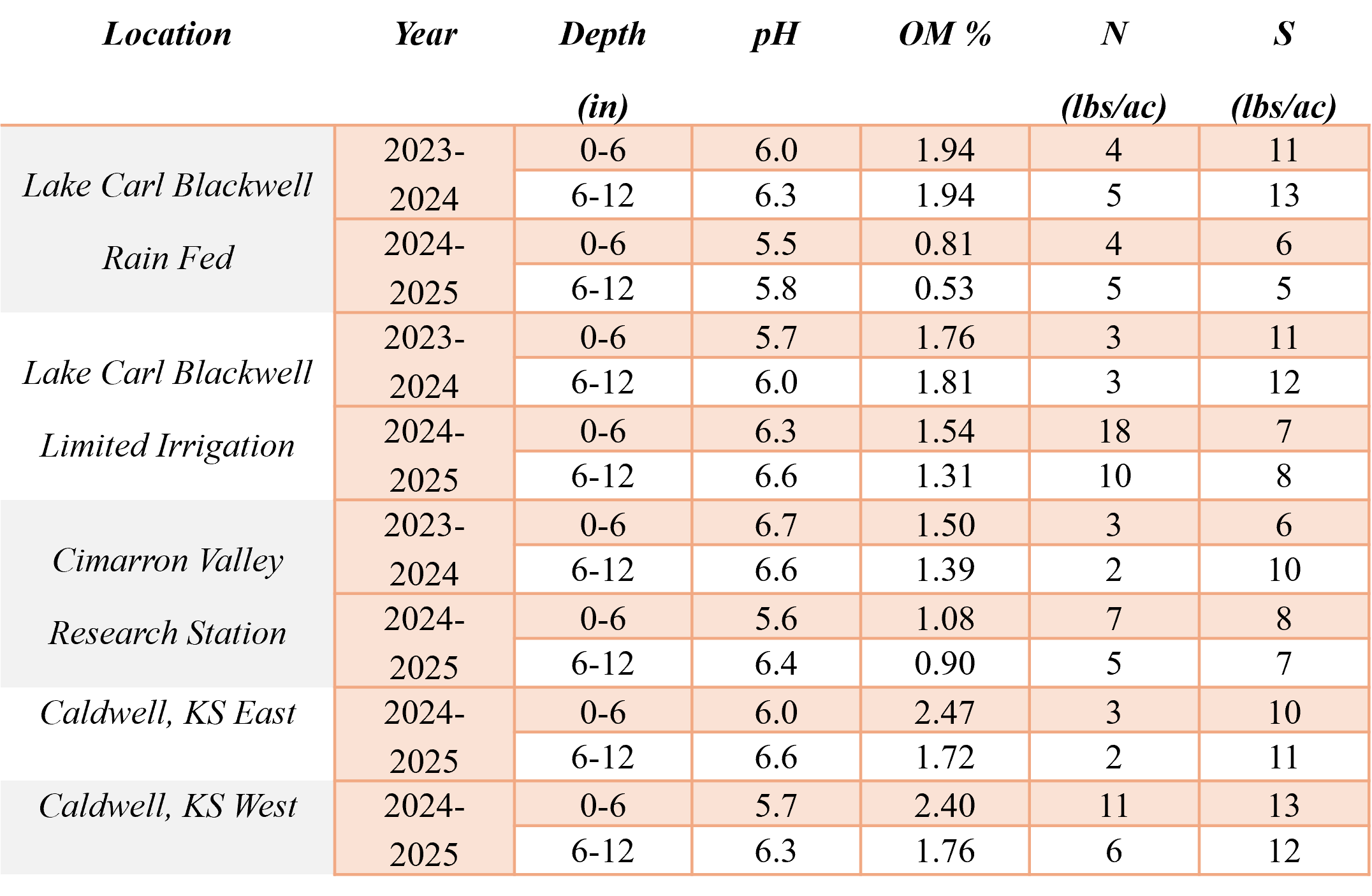
Soil testing was an important part of interpreting the results. Across the locations, sulfate-S was present in the soil profile before fertilizer application. Soil test S varied among sites and depths, reinforcing that the amount of S already available to the crop can differ considerably among fields.
Table 1. Average composite soil sample results of pH, organic matter (OM), nitrate, and SO4 for all locations of the S interaction study.
First, What Happened to Yield?
Nitrogen remained the dominant factor controlling grain yield. Across environments, average wheat yield increased from 46 bu/ac with the lower N rate to 56 bu/ac with the higher N rate. Sulfur, however, did not significantly increase grain yield. Soil tests indicated that the sites generally contained measurable sulfate-S, which correctly predicted the lack of a yield response. If grain yield had been our only measurement, the story could have ended there. But the addition of S affected several characteristics related to how the grain performed during milling and dough development, particularly under the high-N treatment.
Why Wheat Quality Matters
Most Oklahoma wheat producers market wheat based primarily on grain yield and protein concentration. Once wheat moves farther through the grain chain, however, millers and commercial bakeries evaluate additional characteristics that determine how the flour performs. Hard red winter wheat is valued for its ability to produce strong bread flour. That ability depends not only on the amount of protein in the grain but also on the structure and functionality of those proteins. Nitrogen applications generally increases grain protein concentration, while S can influence the composition of those proteins. Adequate S promotes the formation of S-containing proteins involved in strong gluten networks. As a result, two wheat samples with similar protein concentrations can potentially behave differently during milling and baking.
Looking Beyond Grain Protein
Several measurements were used to evaluate wheat and flour quality. Grain protein represents the total protein concentration of the kernel and remains an important factor in wheat marketing. Flour protein measures the protein concentration after the bran and other components have been removed during milling. Other measurements tell us more about milling and baking performance. Milling yield describes how much usable flour can be produced from the grain, while flour ash is an indicator of the amount of mineral material remaining in the flour and can help evaluate milling efficiency. Falling number provides information about alpha-amylase activity and potential preharvest sprouting. Gluten index is particularly useful for evaluating gluten strength. A higher gluten index generally indicates stronger gluten that can better maintain dough structure during mixing and fermentation.
What Happened When We Made Dough?
One of the unique aspects of this study was evaluating flour with DoughLAB analysis. Rather than measuring only grain or flour composition, DoughLAB measures how flour behaves during mixing. Development time measures how long the dough must be mixed to reach optimum consistency. Dough stability measures how long the dough maintains that consistency before beginning to break down. Mixing tolerance index, or MTI, measures how rapidly the dough weakens after optimum development. Water absorption measures the amount of water required to produce dough at a standard consistency.
Of these measurements, dough stability provided one of the more interesting S responses. Under the high-N treatment, average dough stability increased from approximately 6 minutes without S to nearly 15 minutes at the highest S rate. Greater dough stability indicates that the gluten network was able to withstand mixing for a longer period before breaking down. For commercial baking, this can be important because stronger, more stable dough generally provides greater tolerance during mixing and more consistent performance during processing.
What Did We Learn?
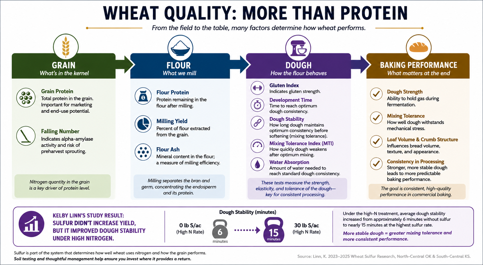
Across these environments, N remained the primary factor controlling grain yield. Increasing N increased average yield, while adding S did not provide a significant yield response. However, the absence of a yield response did not mean S had no effect on the wheat. Under high-N conditions, S improved several measurements associated with grain and dough functionality, including gluten strength, dough development, and dough stability.
These results help separate two questions that are sometimes treated as the same question: Does the crop need S to produce more grain, and does S influence what happens inside the grain?
At the locations included in this study, the answer to the first question was no. The soils supplied enough S that additional fertilizer did not increase yield. The second question was more complicated. Sulfur influenced characteristics associated with protein functionality and end-use quality, particularly when N supply was high. That does not mean S should be applied routinely to improve wheat quality. For producers, the first fertilizer decision should still be based on whether the crop is likely to become S deficient. Soil testing, soil texture, organic matter, yield potential, and production history all provide information that can help make that decision. The larger lesson from this work is that S has a role in wheat beyond simply producing more bushels. Understanding that role helps us make better fertilizer decisions while continuing to put fertilizer where it is most likely to provide a return.
Data drawn from The Influence of Sulfur Under Nitrogen Extremes in Winter Wheat.
Linn, Kelby DeeAnn. Oklahoma State University ProQuest Dissertations & Theses, 2026. 32668685.
Stop the March: Starting Your Wheat Season Off Right with Fall Armyworm Management
Ashleigh M. Faris, State Specialist for Cropping Systems Entomology
As Oklahoma summer crops are winding down, we are seeing an increase in fall armyworm reports. Fall armyworms are posing a significant risk of economic damage to our upcoming winter wheat crop. These summer crops and weeds have supported lush vegetation, creating highly attractive habitats for female moths to lay eggs, which can subsequently move into newly planted wheat.
Here is what wheat producers need to know to identify, manage, and prevent fall armyworm infestations this planting season.
Fall Armyworm (FAW) Identification and Life Cycle
Fall armyworms have a distinct, broad, white inverted “Y” present on the front of their head capsule (Fig. 1). Their body varies from light tan to green to dark brown or nearly black in color with three widely separated narrow, yellowish-white stripes down their back (Fig. 2). There are four distinct black dots arranged in a square on the top of the 8th abdominal segment.

Fig. 1 Fall armyworm. Note the white inverted “Y” on the head capsule. Credit: Mitchell Alcala, OSU Agriculture.
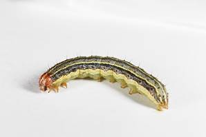
Fig. 2. Fall armyworm. Credit: Pat Porter, Texas A&M AgriLife Extension.
The adult moth will lay their eggs that hatch as caterpillars (the damaging stage). Adult moths migrate from Mexico and Texas to Oklahoma usually by late June. Eggs are laid in clusters on host plants and appear pale yellow but darken as they age turning black just before hatching (Fig. 3). Larvae will feed on foliage for 2-3 weeks, increasing with size as they progress through 6 larval instars, then dig into the soil to pupate. A new generation of moths emerge about 2 weeks later. Because there are several overlapping generations in Oklahoma, extending into October and November, protecting wheat stands and monitoring for FAW can be critical for crop establishment. Keep in mind that FAW do not overwinter in Oklahoma; the first killing frost of the season should eradicate the population.
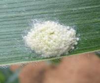
Fig. 3. Fall armyworm eggs laid on grass. The fuzzy appearance is due to scales that are deposited between and over the eggs. Credit: Desiree van Heerden, Syngenta.
Signs of FAW Damage, Scouting, and Economic Threshold
The earliest sign of infestation is “windowpane” damage, where tiny, newly hatched FAW larvae chew off a single layer of leaf tissue, leaving behind transparent patches (Fig. 4). Within a few days, the growing FAW caterpillars can consume entire leaves. Because 90% of crop damage happens during the insect’s final two growth stages, FAW can quickly decimate seedling stands, sometimes forcing producers to completely replant their winter wheat.
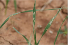
Fig. 4. Small FAW larvae will scrape off the top layer of leaf tissue when they feed, leaving behind a “windowpane” appearance. Credit: Lanie Hale, Wheeler Bros.
To scout for FAW, check your fields regularly (e.g., every other day in the evenings), looking closely at the base of newly emerged seedlings. Focus on field borders and edges near grassy or weedy areas where FAW often start. During the day FAW will hide under residue and at the base of the plant, scouting early morning or in the evenings is the best time for spotting FAW in the crop canopy. Look closely and carefully for early instars, as these are very small (Fig. 5).

Fig. 5. Small, early instar FAW can be difficult to see against wheat and residue, especially when scouting in full sun. Red circles highlight the FAW hiding in this image. Credit: Dr. Amanda Silva, OSU Small Grains Extension Specialist.
The economic threshold for FAW in winter wheat is 3 – 4 larvae per linear foot of row alongside visible feeding damage. Alternatively, treat when there are 4 or more larvae (1 inch or longer) per square foot threatening the stand. If 25-30% of plants show window-pane injury, monitor the field daily and treat immediately if the stand is in danger.
Planting Practices: Cultural Control & Insecticide Seed Treatments
Keeping your field and its surrounding borders completely weed-free, in additional to removal of volunteer wheat for at least two weeks before planting is one way to make sure your wheat season starts off on the right foot. This removes early food sources and makes the area less attractive for egg-laying female moths.
Another way to get your season off on the right foot is to consider using an insecticide seed treatment but make sure it is specifically labeled for FAW. This is because not all insecticides are effective against FAW. Seed treatments containing the active ingredient Chlorantraniliprole (Group 28), such as Cedocor CPL and Lumivia, are effective options labeled to control or suppress FAW. These products also provide protection against wireworms, cutworms, and grasshoppers. Insecticide seed treatments can provide protection for four to six weeks.
How do you know if you should invest in a seed treatment? Consider your planting timing and intended use for your wheat. Planting wheat early for use as a dual-purpose crop significantly increases the prevalence of several diseases and damage caused by viruses, fungi, and by insect pests compared to planting wheat later for grain-only. You should also consider the history of the field. If you have seen issues in a particular field, then it may be worth planting treated seed. If you don’t know the history of the field, work with your local agronomist to determine what insects are likely an issue in those fields.
If you are using treated seed, remember that combinations of some fungicidal and insecticidal seed treatments can be toxic to the seed. Read the label carefully before mixing insecticides with fungicides. Also be sure to follow required grazing restrictions and intervals listed on the label. Equipment such as augers and trucks to deliver grain should not be contaminated by treated grain.
Foliar Chemical Control Options
It is critical to treat fields while FAW caterpillars are on the small side meaning less than half an inch long; larger caterpillars do the most damage and can be highly resilient to insecticides. Effective foliar products typically include active ingredients like chlorantraniliprole, lambda-cyhalothrin, spinetoram, or cyfluthrin. Options labeled for FAW control include Coragen eVo, Tombstone, Warrior II, Mustang Maxx, Besiege, and Radiant SC. When selecting an insecticide, it is important to consider if the option is broad spectrum. Broad spectrum insecticides can reduce natural control such as lacewing and syrphid larvae, as well as lady beetles that may be keeping other pests like aphids under threshold. Always read and follow all label instructions to ensure you are applying at the correct rate and adhering to the required pre-harvest and grazing intervals.
This fall, the OSU Cropping Systems Entomology team will be conducting field trials to evaluate the efficacy of insecticide seed treatments and foliar insecticides on FAW in hard red winter wheat. These trials are made possible through support from industry partners and the Oklahoma Wheat Commission. Trial results will be shared at future OSU Field Days and grower meetings.

