Home » Fertilizer
Category Archives: Fertilizer

The Mechanics of Soil Fertility: Use of Sugar in Field Crops
Jolee Derrick, Precision Nutrient Management Ph. D. Student
Grace Williams, Soil Microbiology Ph. D. Candidate
Brian Arnall, Precision Nutrient Management Specialist
Recently, there has been increased interest in adding sugar to spray tank mixes, whether for post-emergence weed control or foliar nutrient applications. While there is limited work on impact of sugar inclusion in herbicide applications, some papers have posed potential enhancement (Devine and Hall, 1990). But since this is coming from a soil science group, we will only focus on soil impact. Following up the last blog, unlike humic substances, which represent more complex and relatively stable carbon forms, sugar is a highly labile carbon source. This rapid utilization of simple carbon sources is well documented to stimulate microbial activity and growth (Kuzyakov and Blagodatskaya, 2015). The general idea of utilizing sugar applications is that sugar has the capacity to improve spray performance, stimulate biological activity, increase organic matter mineralization, and ultimately result in improved yields.
Sugar additions can influence soil processes differently depending on system conditions. In systems with higher residual nitrogen and organic matter, responses may differ from those observed in Oklahoma production environments, where soils are typically lower in organic matter and microbial activity can occur for much of the year. Understanding how sugar functions in these systems requires a basic discussion of carbon dynamics. Sugar itself is almost entirely carbon and is readily consumed by microbes. It’s a simple molecule, which allows it to dissolve easily in water and be quickly utilized in the soil system. Crop residues, like wheat straw, are also carbon-rich but much more complex. They contain cellulose, hemicellulose, and lignin which are long carbon chains that take time to break down because microbes need specialized enzymes to access them.
For the sake of simplicity, we can group carbon into two key pools: labile carbon and particulate organic matter (POM). Labile carbon includes easily decomposed materials, which include the previously mentioned simple sugars that microbes can metabolize rapidly. These pools differ in turnover time and microbial accessibility, with labile carbon driving short-term microbial responses (Cotrufo et al. 2013). POM breaks down more slowly and serves as a longer-term nitrogen source through residue breakdown.
Soil microorganisms require both carbon and nitrogen to grow and maintain biomass, typically at a ratio of approximately 24 parts carbon to 1 part nitrogen. When readily available carbon is abundant, but nitrogen is limited, microbes increase their nitrogen demand and begin scavenging nitrogen from the surrounding soil. This process, better known as nitrogen immobilization, temporarily reduces nitrogen availability to crops. Additions of readily available carbon sources have consistently been shown to increase microbial nitrogen immobilization in soil systems (Recous et al. 1990).
In systems where sufficient nitrogen is present, microbial populations can expand rapidly. Fast-growing microbial species may dominate, continuing to immobilize nitrogen within their biomass. Eventually, when nitrogen becomes limiting, microbial populations decline to levels the system can support. This boom-and-bust cycle can disrupt nitrogen availability during critical stages of crop growth. These rapid shifts in microbial population and activity following carbon inputs are commonly observed in soil systems receiving easily decomposable substrates (Blagodatskaya and Kuzyakov, 2008).
This dynamic becomes especially relevant when considering residue management practices common in Oklahoma. Under no-till or limited-tillage systems, the crop residues have wide carbon-to-nitrogen (C:N) ratios, creating conditions where nitrogen immobilization can occur during the growing season.
Table 1 provides approximate C:N ratios for several crops commonly grown in Oklahoma. When additional carbon is introduced into these systems without accompanying nitrogen, the likelihood of microbial immobilization increases. While immobilization is not bad, it does create a question mark as Oklahoma’s variable climate means the following release of nutrients will be unpredictable.
Table 1. Table depicting the range of C:N ratios for residues of commonly utilized crops in Oklahoma. Ratios were obtained from Brady, N. C., & Weil, R. R. (2017). The Nature and Properties of Soils (15th ed.)

Now consider conventional tillage systems. In Oklahoma, no-till systems typically contain 2 to 3 percent organic matter, which is relatively high given our climate and extended periods of microbial activity. Conventional tillage systems often fall between 0.75 and 2.25 percent organic matter. Because soil organic matter is approximately 58 percent carbon, this represents a substantial difference in the soil carbon pool.
Tillage can temporarily enhance microbial access to both previously mentioned carbon pools. When tillage exposes previously protected carbon, microbial activity increases rapidly. This initial flush can temporarily increase nitrogen mineralization as organic nitrogen is converted to plant-available forms. However, this phase is short-lived. As microbial populations expand, nitrogen demand increases, leading to immobilization and reduced nitrogen availability.
Hypothetically, increased microbial growth and activity would rapidly mineralize organic matter, trigger a surge in NO₃⁻, deplete soil organic matter, and as resources become limiting and the environment can no longer sustain elevated microbial populations, this boom would be followed by a population crash. This relationship is ultimately driven by the soil C:N ratio, which introduces an interesting additional complexity of residue. Different residues bring very different carbon-to-nitrogen balances into the system, and microbes respond accordingly. High carbon residues give microbes plenty of energy but very little nitrogen, so they pull N out of the soil to meet their needs. Residues with lower C:N ratios (soybean, alfalfa, etc.) do opposite, releasing nitrogen as they break down. Now the real question becomes where the critical point sits, and when does management push the system from the threshold of immobilization and mineralization.
These hypotheses form the foundation for new research currently underway through the Precision Nutrient Management Program. Initial proof-of-concept work has already been completed, providing a necessary steppingstone to address these questions.
Figure 1. Graph depicting the different concentrations of nitrate leached corresponding to applied treatments in the proof-of-concept work
The preliminary work (Figure 1) evaluated different sugar sources applied alongside a high-nitrogen product to assess the extent of nitrogen immobilization. Although these studies were conducted using potting soils, clear trends were apparent. Treatments containing sugar consistently showed greater nitrogen immobilization compared to treatments without sugar. This response is consistent with studies showing that additions of simple carbon substrates stimulate microbial growth and increase nitrogen immobilization (Dendooven et al. 2006). Building on this work, an active field-based research project is underway to evaluate how sugar additions influence nitrogen availability and microbial dynamics under real-world Oklahoma production conditions.
From an agronomic standpoint, sugar functions primarily as a readily available carbon source that stimulates microbial growth. In nitrogen-limited systems, this response increases the likelihood that nitrogen will be incorporated into microbial biomass rather than remaining immediately available for crop uptake.
Finally, we conclude with a conceptual consideration. If increased OM mineralization leads to greater plant biomass, this process may partially offset losses of OM. Greater biomass production could return more residues to the soil, contributing to the OM pool in the upper soil profile. Therefore, the system may compensate for OM mineralization through the rebuilding of organic matter via plant inputs. However, the stabilization of this carbon depends on microbial processing and physical protection within the soil matrix (Cotrufo et al. 2015)
However, while the underlying logic is sound, this concept has not been extensively studied within Oklahoma cropping systems. This blog does not address the impact of sugar applications on residue breakdown, and the potential impact of such. Future research through the Precision Nutrient Management Program will further investigate the mineralization process to better understand carbon dynamics within these systems.
Take Home:
- Oklahoma production systems generally have lower residual N and high carbon residues, creating conditions conducive to N immobilization
- Adding sugar increases microbial growth, creating population booms that will momentarily increase mineralization, but then immediately immobilize residual nitrogen.
- Tillage can amplify the negative effects of sugar by exposing more carbon and reducing soil organic matter
- Proof-of-concept work shows sugar triggered a net nitrogen immobilization in a carbon heavy environment
- Proof-of-concept work also suggests that when additional nitrogen is present, sugar additions may shift the system toward net mineralization rather than immobilization.
Work Cited:
Blagodatskaya, E., & Kuzyakov, Y. (2008). Mechanisms of real and apparent priming effects. Biology and Fertility of Soils, 45, 115–131.
Brady, N. C., and R. R. Weil. “The Nature and Properties of Soils, 15th Edn (eBook).” (2017).
Cotrufo, M. F., Wallenstein, M. D., Boot, C. M., Denef, K., & Paul, E. (2013). The Microbial Efficiency-Matrix Stabilization (MEMS) framework. Global Change Biology, 19, 988–995.
Cotrufo, M. F., Soong, J. L., Horton, A. J., Campbell, E. E., Haddix, M. L., Wall, D. H., & Parton, W. J. (2015). Formation of soil organic matter via biochemical and physical pathways of litter mass loss. Nature Geoscience, 8(10), 776–779.
Dendooven, L., Verhulst, N., Luna-Guido, M., & Ceballos-Ramírez, J. M. (2006). Dynamics of inorganic nitrogen in nitrate- and glucose-amended alkaline–saline soil. Plant and Soil, 283(1–2), 321–333.
Devine, M. D., & Hall, L. M. (1990). Implications of sucrose transport mechanisms for the translocation of herbicides. Weed Science, 38(3), 299–304.
Kuzyakov, Y., & Blagodatskaya, E. (2015). Microbial hotspots and hot moments in soil: Concept & review. Soil Biology and Biochemistry, 83, 184–199.
Recous, S., Mary, B., & Faurie, G. (1990). Microbial immobilization of ammonium and nitrate in cultivated soils. Soil Biology and Biochemistry, 22, 913–922.
Mechanics of Soil Fertility: Understanding Humic and Fulvic Acids
Brian Arnall, Oklahoma State University, Precision Nutrient Management Extension Specialist
Oliver Li, Oklahoma State University, Soil Chemistry
Interest in humic and fulvic acid products has increased substantially in agricultural production systems during the past two decades. These materials are frequently promoted as tools for improving soil biology, increasing nutrient availability, enhancing fertilizer efficiency, and stimulating plant growth. Because humic substances are known to be important components of soil organic matter, it is reasonable to ask whether adding humic or fulvic products to soil can meaningfully influence soil fertility.
As with many soil fertility questions, the answer depends on understanding two key factors: the mechanism involved and the magnitude of that mechanism relative to the soil system. Soil processes operate within large natural pools of organic matter, nutrients, and microbial activity. Therefore, evaluating the potential effects of humic products requires examining both how these compounds function chemically and biologically and how their application rates compare with the soils organic matter.
What Are Humic and Fulvic Acids?
Humic substances are heterogeneous organic compounds formed during the decomposition and transformation of plant and microbial residues. Historically, soil scientists have divided these materials into three operational fractions based on their solubility behavior: humic acid, fulvic acid, and humin (Stevenson, 1994; Tan, 2014). Humic acids are relatively large molecules that are insoluble under acidic conditions but dissolve in alkaline solutions. Fulvic acids are smaller molecules that remain soluble across the entire pH range, which allows them to move more freely in soil solution.
Both humic and fulvic acids contain numerous functional groups, particularly carboxyl and phenolic groups, which carry negative charge. These functional groups allow humic substances to interact with metal ions and nutrient cations and contribute to several important soil properties, including cation exchange capacity, buffering capacity, and metal complexation (Stevenson, 1994; Lehmann and Kleber, 2015). Because these materials originate from decomposed organic residues, they represent one portion of the complex mixture that collectively makes up soil organic matter. The distribution of the soil organic matter fractions varies among soil types and land uses, but fulvic acids and humic acids are each typically estimated to comprise approximately 10–35% of total soil organic matter (Guimarães et al., 2013).
Nutrient Retention and the Role of Cation Exchange
One of the most commonly cited mechanisms associated with humic substances is their ability to retain nutrients through cation exchange. The negatively charged functional groups present on humic molecules attract positively charged ions in soil solution. Through this electrostatic attraction, humic materials can retain several plant nutrients, including ammonium, potassium, calcium, magnesium, and certain micronutrients such as zinc and copper (Stevenson, 1994; Tan, 2014). This mechanism functions in the same manner as cation exchange on clay minerals. Of course, negatively charged surfaces do not retain negatively charged ions. As a result, nutrients such as nitrate are not held by humic substances and remain mobile in soil solution.
Laboratory measurements indicate that humic materials may possess relatively high cation exchange capacity on a mass basis. Reported values commonly range from approximately 300 to 600 cmolc kg⁻¹ depending on the source material and extraction method (Stevenson, 1994; Tan, 2014). These values demonstrate that humic substances can retain a large amount of cationic nutrients. A question that can be posed, however, is how this capacity compares with the nutrient retention already provided by soil organic matter.
Understanding the magnitude of humic additions requires comparing product application rates with the organic matter already present in soil. Calculations based on typical cation exchange values suggest that one pound of humic material with a CEC of 300–600 cmolc kg⁻¹ could theoretically retain approximately 0.04 to 0.08 pounds of ammonium-nitrogen. When viewed in isolation this number may appear meaningful. However, agricultural soils already contain large quantities of organic matter. An acre furrow slice, representing approximately the upper six inches of soil, weighs roughly two million pounds. Soil containing one percent organic matter therefore contains about 20,000 pounds of organic material per acre (Brady and Weil, 2016). Humified organic matter typically has cation exchange capacities ranging between 150 and 300 cmolc kg⁻¹ (Stevenson, 1994), meaning that the exchange capacity associated with native soil organic matter is already substantial. To put this into perspective, one pound of humic material can retain roughly 0.04 to 0.08 pounds of cation charge. Ammonium and potassium carry a single positive charge, while calcium carries two, meaning two ammoniums can be held for every two calcium. To provide contrast to the application of a humic substance, increasing soil organic matter by just 0.1% equivalent to about 2,000 pounds of additional organic material per acre can provide the capacity to retain approximately 40 to 80 pounds of cation charge or 40 to 80 pounds of ammonium.
The key point is not that humic materials cannot retain nutrients. They clearly can. Rather, the scale of material already present in soil is extremely large compared with the few ounces or pounds of humic products typically applied in agricultural systems. Consequently, the nutrient retention capacity associated with soil organic matter overwhelmingly dominates the soil system.
Micronutrient Complexation
Humic and fulvic substances are also known to interact with micronutrients through metal complexation reactions (also known as ‘chelation’). Carboxyl and phenolic functional groups can coordinate with metal ions such as iron, zinc, copper, and manganese to form organic complexes (Stevenson, 1994; Tan, 2014). These complexes can influence micronutrient mobility and availability in soils.
Fulvic acids are particularly effective at forming soluble complexes because they remain dissolved across the full range of soil pH. In some cases, these complexes may increase micronutrient mobility and transport within the soil solution. This mechanism has been well documented in soil chemistry research and may explain some responses observed in systems where micronutrient availability is limited.
Effects on Plant Physiology
In addition to soil chemical interactions, humic substances may influence plant growth through physiological mechanisms occurring in the rhizosphere. Several studies have shown that humic substances can stimulate root development, including increases in root elongation, lateral root formation, and root hair production (Nardi et al., 2002; Canellas and Olivares, 2014).
Research suggests that these responses may involve interactions with plant hormonal pathways and membrane transport processes. Humic substances have been shown to activate plasma membrane H⁺-ATPase enzymes, which are involved in proton pumping and nutrient uptake across root membranes (Canellas et al., 2002; Trevisan et al., 2010). Activation of these transport systems can enhance nutrient absorption and influence root architecture.
These physiological effects appear to occur primarily at the root–soil interface, where dissolved organic molecules interact directly with plant tissues. As a result, the responses observed in plant growth experiments are often attributed to rhizosphere signaling processes rather than large changes in bulk soil fertility.
Microbial Responses to Humic and Fulvic Compounds
Soil microorganisms respond strongly to carbon availability, and different carbon sources can produce very different microbial responses. Simple carbohydrates such as glucose and sucrose are readily metabolized by soil microbes and therefore produce rapid increases in microbial respiration and biomass. Humic substances, in contrast, consist of chemically complex and partially oxidized organic compounds that decompose much more slowly (Lehmann and Kleber, 2015).
Experimental studies comparing carbon sources consistently show that microbial respiration increases dramatically when simple sugars are added to soil, whereas humic substances produce smaller responses (Blagodatskaya and Kuzyakov, 2008). This difference reflects the relative degradability of these compounds as microbial energy sources.
Carbon Inputs from Humic Products Compared with Natural Soil Carbon
Soil microbial activity is largely driven by carbon supplied from plants through root exudation, residue decomposition, and organic matter turnover. The carbon pools already present in soil are therefore important for understanding the potential influence of humic product additions. A soil containing one percent organic matter holds approximately 11,600 pounds of carbon per acre (Brady and Weil, 2016).
Research on plant–soil carbon cycling indicates that living roots release significant quantities of organic carbon into soil each growing season through root exudation and rhizodeposition (Kuzyakov and Domanski, 2000). These plant-derived carbon inputs commonly amount to hundreds of pounds of carbon per acre and serve as a major energy source for soil microbial communities. Viewed in this context, humic product applications represent extremely small additions to the soil carbon pool. Consequently, microbial stimulation in agricultural soils is dominated by carbon inputs from plant residues and root exudates rather than by small additions of humic materials.
Building Organic Matter in the Central Plains
Increasing soil OM in the central Great Plains is achievable, but the magnitude of change is governed primarily by carbon inputs and water availability rather than any single management practice. Systems that combine no-till, increased residue return, diversified crop rotations, and where feasible cover crops or manure inputs are the most effective because they simultaneously increase carbon inputs and reduce decomposition losses (Lyon et al., 2007; Mikha et al., 2013; Nielsen et al., 2016). In semi-arid systems, realistic rates of OM increase are modest: over a 5-year period, changes are often small, approximately +0.05 to 0.1% OM, but significant in relation to the system which is often at total OM levels between 0.7 and 1.25 prior to establishment of conservation practices. The increase is confined to the top inch of the soil surface (Mikha et al., 2013; Saha et al., 2024). Mechanistically, these gains occur through greater residue and root-derived carbon inputs, reduced soil disturbance which slows microbial oxidation, and improved aggregation that physically protects organic matter from decomposition (Six et al., 2002; Lehmann and Kleber, 2015). However, as emphasized throughout this discussion, the scale of change is small relative to the large existing organic matter pool, and meaningful increases require long-term, system-level management focused on maximizing biomass production rather than relying on small external carbon additions such as commercial products.
Take-Home Points
- Humic and fulvic acids can retain cations, chelate micronutrients, and influence plant and microbial processes.
- Typical application rates are small relative to existing soil organic matter, so whole-soil impacts are limited.
- Most observed effects are localized in the rhizosphere, not broad changes in soil fertility.
- Evaluating both mechanism and scale is key to understanding their role in nutrient management.
References
Blagodatskaya, E., & Kuzyakov, Y. (2008). Mechanisms of real and apparent priming effects and their dependence on soil microbial biomass and community structure. Biology and Fertility of Soils, 45(2), 115–131.
Brady, N. C., & Weil, R. R. (2016). The nature and properties of soils (15th ed.). Pearson.
Canellas, L. P., Olivares, F. L., Okorokova-Façanha, A. L., & Façanha, A. R. (2002). Humic acids isolated from earthworm compost enhance root elongation and lateral root emergence in maize. Plant Physiology, 130(4), 1951–1957.
Canellas, L. P., & Olivares, F. L. (2014). Physiological responses to humic substances as plant growth promoters. Chemical and Biological Technologies in Agriculture, 1, 3.
Guimarães, D. V., Gonzaga, M. I. S., Silva, T. O., Silva, T. L., Dias, N. S., & Matias, M. I. S. (2013). Soil organic matter pools and carbon fractions in soil under different land uses. Soil and Tillage Research, 126, 177–182.
Kuzyakov, Y., & Domanski, G. (2000). Carbon input by plants into the soil: Review. Journal of Plant Nutrition and Soil Science, 163(4), 421–431.
Lehmann, J., & Kleber, M. (2015). The contentious nature of soil organic matter. Nature, 528(7580), 60–68.
Lovley, D. R., Coates, J. D., Blunt-Harris, E. L., Phillips, E. J. P., & Woodward, J. C. (1996). Humic substances as electron acceptors for microbial respiration. Nature, 382, 445–448.
Lyon, D. J., Stroup, W. W., & Brown, R. E. (2007). Crop production and soil water storage in long-term winter wheat–fallow tillage experiments. Soil and Tillage Research, 94(2), 387–397.
Mikha, M. M., Vigil, M. F., Benjamin, J. G., & Sauer, T. J. (2013). Cropping system influences on soil carbon and nitrogen stocks in the Central Great Plains. Soil Science Society of America Journal, 77(2), 702–710.
Nardi, S., Pizzeghello, D., Muscolo, A., & Vianello, A. (2002). Physiological effects of humic substances on higher plants. Soil Biology and Biochemistry, 34(11), 1527–1536.
Nielsen, D. C., Lyon, D. J., Hergert, G. W., Higgins, R. K., Calderón, F. J., & Vigil, M. F. (2016). Cover crop mixtures do not use water differently than single-species plantings. Agronomy Journal, 108(3), 1025–1038.
Saha, D., Kukal, S. S., & Bawa, S. S. (2024). Long-term impacts of conservation agriculture practices on soil organic carbon and aggregation. Soil Science Society of America Journal.
Six, J., Conant, R. T., Paul, E. A., & Paustian, K. (2002). Stabilization mechanisms of soil organic matter: Implications for C saturation of soils. Plant and Soil, 241(2), 155–176.
Stevenson, F. J. (1994). Humus chemistry: Genesis, composition, reactions (2nd ed.). Wiley.
Tan, K. H. (2014). Humic matter in soil and the environment. CRC Press.
Trevisan, S., Francioso, O., Quaggiotti, S., & Nardi, S. (2010). Humic substances biological activity at the plant–soil interface. Plant Signaling & Behavior, 5(6), 635–643.
For any questions or commments please feel free to reach out to Brian Anrall, b.arnall@okstate.edu
One Well-Timed Shot: Rethinking Split Nitrogen Applications in Wheat production
Brian Arnall, Precision Nutrient Management Specialist
Samson Abiola, PNM Ph.D. Student.
Nitrogen is the most yield limiting nutrient in wheat production, but it’s also the most unpredictable. Apply it too early, and you risk losing it to leaching or volatilization before your crop can use it. Apply it too late, and your wheat has already determined its yield potential; you’re just feeding protein at that point. For decades, the conventional wisdom has been to split nitrogen applications: put some down early to get the crop going, then come back later to apply again. But does splitting actually work? And more importantly, when is the optimal window to apply nitrogen if you want to maximize both yield and protein quality? We spent three years across different Oklahoma locations testing every timing scenario to answer these questions.
How We Tested Every Nitrogen Timing Scenario in Oklahoma Wheat
Between 2018 to 2021, we conducted field trials at three Oklahoma locations, including Perkins, Lake Carl Blackwell, and Chickasha, representing different soil types and growing conditions across the state. We tested three nitrogen rates: 0, 90, and 180 lbs N/ac, applied as urea at five critical growth stages based on growing degree days (GDD). These timings were 0 GDD (preplant, before green-up), 30 GDD (early tillering), 60 GDD (active tillering), 90 GDD (late tillering, approximately Feekes 5-6), and 120 GDD (stem elongation, approaching jointing). We also compared single applications at each timing against split applications, where half the nitrogen (45 lbs N ac-1) went down preplant, and the other half was applied in-season (45 lbs N ac-1).
The Sweet Spot: Yield and Protein at the 90 lbs N/ac Rate
Across all site-years, at the 90 lbs N/ac rate, timing had a significant impact on both yield and protein. The highest yields came from the 30 and 90 GDD timings, producing 62 to 66 bu/ac, with 60 GDD reaching the peak (Figure 1). Protein at these early timings stayed relatively modest at 13%. The 90 GDD timing delivered 62 bu/ac with 14% protein matching the yield of the 30 GDD application but pushing protein a percentage higher (Figure 2). The real problem appeared at 120 GDD. Delaying application until stem elongation dropped yields to just 49 bu/ac, even though protein climbed to 15%. That’s a 13 bushel penalty compared to the 90 GDD timing. At current wheat prices per bushel, that late application may cost farmers over $100 per acre in lost revenue. By 120 GDD, the crop has already determined its yield potential tillers are set, head numbers are locked in and nitrogen applied at this stage can only be directed toward protein synthesis, not building more yield components.
More Nitrogen Does not lead to high yield
Doubling the nitrogen rate to 180 lbs N/ac revealed something critical, more nitrogen doesn’t mean more yield. The yield pattern remained nearly identical to the 90 lbs N/ac rate. The 60 GDD timing produced the highest yield at 68 bu/ac, followed closely by 30 GDD at 67 bu/ac. The 90 GDD timing yielded 62 bu/ac, and the 120 GDD timing again crashed to 51 bu/ac. The only difference between the two rates was protein concentration (Figure 2). At 180 lbs N/ac, protein levels increased across all timings: 13% at preplant, 15% at both 30 and 60 GDD, 15-16% at 90 GDD, and 16% at 120 GDD. This confirms a fundamental principle: once farmers supply enough nitrogen to maximize yield potential, which occurred at 90 lbs N/ac in these trials, additional nitrogen only increases grain protein. It does not build more bushels. Unless farmers are receiving premium payments for high-protein wheat, that extra 90 lbs of nitrogen represents a cost with no yield return.

Should farmers split their nitrogen application?
Now that timing has been established as critical, the next question becomes: should farmers split their nitrogen applications, or is a single application sufficient? The conventional recommendation has been to split nitrogen apply part preplant to support early growth and tillering, then return with a second application later in the season to boost protein and finish the crop. But does the data support this practice? We compared three strategies at each timing: applying all nitrogen preplant, applying all nitrogen in-season at the target timing, or splitting nitrogen equally between preplant and in-season timing. The goal was to determine whether the extra trip across the field will deliver better results.
Our findings revealed that splitting provided no consistent advantage. At 30 GDD, all three strategies preplant, in-season, and split performed identically, producing 62-65 bu/ac with 12-13% protein (Figure 3 and 4). No statistical differences existed among them. At 60 GDD, similar pattern was held. Yields ranged from 61 to 66 bu/ac and protein stayed at 12-13% regardless of whether farmers applied all nitrogen preplant, all at 60 GDD, or split between the two. At 90 GDD, the single in-season application actually outperformed the split. While yields remained similar across all three methods (61-64 bu/ac), the in-season application delivered significantly higher protein at 13.7% compared to 12.4% for preplant and 12.5% for split applications. This suggests that concentrating nitrogen at 90 GDD, rather than diluting it across two applications, allows more efficient incorporation into grain protein. The only timing where splits appeared beneficial was 120 GDD, where the split application yielded 59 bu/ac compared to 51 bu/ac for the single late application. But this is not a win for splitting, it simply demonstrates that applying all nitrogen at 120 GDD is too late and putting half down earlier salvages some of the yield loss. Across all timings tested, splitting nitrogen into two applications offered no agronomic advantage over a single well-timed application, meaning farmers are making an extra pass for no gain in yield or protein.


Practical Recommendations for Nitrogen Management
Based on three years of field data, farmers should target the 90 GDD timing (late tillering, Feekes 5-6) for their main nitrogen application to achieve the best balance between yield and protein. This window typically falls in late February to early March in Oklahoma, though farmers should monitor crop development rather than relying solely on the calendar apply when wheat shows multiple tillers, good green color, and vigorous growth. A rate of 90 lbs N/ac maximized yield in these trials; higher rates only increased protein without adding bushels, so farmers should only exceed this rate if receiving premium payments for high-protein wheat. Splitting nitrogen applications provided no advantage at any timing, meaning a single well-timed application at 90 GDD is sufficient for most Oklahoma wheat production systems. The exception would be sandy soils with high leaching potential, where splitting may reduce nitrogen loss. Farmers should avoid delaying applications until 120 GDD or later, as this timing consistently resulted in 15-25 bushel per acre yield losses even though protein increased. For farmers specifically targeting premium protein markets, a two-step strategy works best: apply 90 lbs N/ac at 90 GDD to establish yield potential and baseline protein, then follow with a foliar application of 20-30 lbs N/ac at flowering to push protein above 14% without sacrificing yield. Finally, weather conditions matter hot, dry forecasts increase volatilization risk and reduce uptake efficiency, so farmers should consider moving applications earlier if low humidity conditions are expected.
Split Application Caveat * Note from Arnall.
The caveat to the it only takes one pass, is high yielding >85+ bpa, environments. In these situation I still have not found any value for preplant nitrogen application. I have seen however a split spring application is valuable. Basically putting on 30-50 lbs at green-up, with the rest following at jointing (hollowstem). The method tends to reduce lodging in the high yielding environments.
This work was published in Front Plant Sci. 2025 Nov 6;16:1698494. doi: 10.3389/fpls.2025.1698494
Split nitrogen applications provide no benefit over a single well timed application in rainfed winter wheat
Another reason to N-Rich Strip.
Yet just one more data set showing the value of in-season nitrogen and why the N-Rich Strip concept works so well.
Questions or comments please feel free to reach out.
Brian Arnall b.arnall@okstate.edu
Acknowledgements:
Oklahoma Wheat Commission and Oklahoma Fertilizer Checkoff for Funding.
What OK Cotton Growers Should Know about the Two-Spotted Cotton Leafhopper, aka Cotton Jassid
Ashleigh M. Faris, OSU Extension Cropping Systems Entomologist Department of Entomology and Plant Pathology Oklahoma State University
Jenny Dudak, OSU Extension Cotton Specialist, Department of Plant & Soil Sciences Oklahoma State University
Maxwell Smith, OSU IPM for Cotton Extension Specialist Department of Entomology and Plant Pathology, Oklahoma State University
Published 8.29.25
The two-spotted cotton leafhopper, also known as the cotton jassid (Amrasca biguttula), has not been detected in Oklahoma cotton production as of August 27, 2025. However, this insect pest has been confirmed to be causing significant injury in cotton fields that have high populations of the jassid throughout the southeastern United States (Figure 1). Although it is not known to currently be in Oklahoma cotton acres, our cotton growers and consultants are encouraged to keep an eye out for this pest and to report sightings of the insect or related damage to the OSU Cotton Extension team for confirmation.

Two-Spotted Cotton Leafhopper Identification & Injury
Cotton jassids are small, sap-sucking insects that are pale green insects with yellowish-green wings. They can be distinguished from most native North American species by the pair of black spots head and black spots on the tip of each wing (Figure 2). The immature nymph stages are even smaller than the adults; they are wingless but light green in color like the adults. (Figures 3 and 4).


The cotton jassid feeds on the underside of leaves, causing hopperburn—a rapid yellowing, reddening, and browning that can quickly weaken plants (Figure 5). Initially, injury symptoms may look like nutrient deficiency with slight yellowing along the leaf tips and margins. Injury may also present as upward curling/cupping of the leaves. Once early symptoms are visible, leaves decline rapidly, turning red and brown. Because late-stage hopperburn can resemble a spider mite infestation, growers and consultants should scout for the pest causing injury prior to initiating control. Cotton jassid populations and hopperburn symptoms usually begin on field edges before moving into the cotton field.
Suggested Threshold, Scouting, and Chemical Control Guidance
Current recommendations for the suggested threshold and chemical control options are based on insecticide trials conducted by University of Florida, University of Georgia, Clemson University, and the University of Auburn Extension Entomologists. The threshold at which treatment is recommended for the cotton jassid is 2 nymphs per leaf with injury present anywhere in the field. To scout, inspect the underside of the main stem leaf on the third, fourth, or fifth node from the top of the cotton plant. Sample a minimum of 25 leaves across plants and average counts across the number of leaves sampled.
In terms of management, multiple products seem to provide good efficacy. Bidrin (6 oz/a) has been consistent in multiple trials across Florida, Georgia, and South Carlina, but may be difficult if whiteflies are an issue. Centric (2 oz/a) and Transform (1.5 oz/a) seem to be consistent as well. One product that should not be used is Bifenthrin, which has proven not to be effective across multiple trials. Information on suggested chemical control options, their efficacy, and general IPM guidance will be forthcoming as more is learned about this pest in U.S. cotton systems.
If you detect the cotton jassid in Oklahoma cotton, please contact
IPM for Cotton Extension Specialist Maxwell Smith,
PRE-EMERGENT RESIDUAL HERBICIDE ACTIVITY ON SOYBEANS, 2025
Liberty Galvin, Weed Science Specialist
Karina Beneton, Weed Science Graduate Student.
Objective
Determine the duration of residual weed control in soybean systems following the application of Preemergent (PRE) herbicides when applied alone and in tank-mix combination.
Why we are doing the research
PRE herbicides offer an effective means of suppressing early-season weed emergence, thereby minimizing competition during the critical early growth stage. However, evolving herbicide resistance and the need for longer-lasting weed suppression underscore the importance of evaluating multiple modes of action and their residual properties alone and tank-mixed.
Field application experimental design and methods
Field experiments were conducted in 2022, 2023, and 2024 growing seasons in Bixby, Lane, and Ft. Cobb FRSU Research Stations across Oklahoma. Each herbicide (listed in Table 1) was tested individually, in 2-way combinations, 3-way mixtures, and finally as 4-way combinations that included all active ingredients listed at the label rate.

Soybeans were planted at rates between 116,000 and 139,000 seeds/acre from late May to early June, depending on the year and location. The variety used belongs to the indeterminate mid- maturity group IV, with traits conferring tolerance to glyphosate (group 9 mode of action), glufosinate (group 10), and dicamba (group 4). Not all soybean varieties have metribuzin tolerance. Please read the herbicide label and consult your seed dealer for acquiring tolerant varieties. Row spacing was 76 cm at Bixby and Lane, and 91 cm at Fort Cobb. PRE treatments were applied immediately after planting at each experimental location.
POST applications consisted of a tank-mix of dicamba (XtendiMax VG® – 22 floz/acre), glyphosate (Roundup PowerMax 3®- 30 floz/acre), S-metolachlor (Dual II Magnum® – 16 floz/acre), and potassium carbonate (Sentris® – 18 floz/acre). Applications were made on different dates, mostly after the first 3 weeks following PRE treatments. These timings were based on visual weed control ratings, particularly for herbicides applied alone or in 2-way combinations, which showed less than 80% control at those early evaluation dates. The need for POST applications also depended on the species present at each site, with most fields being dominated by pigweed, as illustrated in the figure below.
Results
Tank-mixed PRE herbicide combinations generally provided superior residual control compared to a single mode of action application (Shown in Figure 1). Timely post-emergent (POST) herbicide applications helped sustain high levels of weed suppression, particularly as the effectiveness of residual PRE declined.

Residual control of tank-mixed PRE
Some herbicides applied alone or in simple 2-way mixes, such as sulfentrazone + chloransulam- methyl and pyroxasulfone + chloransulam-methyl required POST applications within 20 to 29 days after PRE, indicating moderate residual control.
In contrast, 2-way combinations containing metribuzin, such as sulfentrazone + metribuzin and pyroxasulfone + metribuzin, extended control up to 50 days after PRE in some cases, highlighting metribuzin’s importance even in less complex formulations.
Furthermore, 3-way and 4-way combinations including metribuzin provided the longest-lasting control, delaying POST applications up to 51–55 days after PRE.
Injury of specific weeds
Palmer amaranth (Amaranthus palmeri) control in Bixby was consistently high (≥90%) at 2 weeks after PRE in 2022 and 2024 across all treatments. At 4 WAPRE, treatments containing metribuzin alone or in combination maintained strong control (90% or greater).
Texas millet (i.e., panicum; Urochloa texana) and large crabgrass (Digitaria sanguinalis) were effectively managed with most treatments delivering over 90% control early in the season and maintaining performance throughout. In 2024, control remained generally effective, though pyroxasulfone alone showed a temporary lack of control for Texas millet, and single applications declined in effectiveness against large crabgrass later in the season. These reductions were likely due to continuous emergence and the natural decline in residual herbicide activity due to weather. The most consistent late-season control for both species came from 3- and 4-way herbicide combinations.
Morningglory (Ipomoea purpurea) control reached full effectiveness (100%) only when POST herbicides were applied, across all years and locations. Their late emergence beyond the residual window of PRE herbicides reinforces the importance of sequential herbicide applications for season-long control.
Take home messages:
- Incorporating PRE and POST herbicides slows the rate of herbicide resistance
- Tank mixing with *different modes of action* ensures greater weed control by having activity on multiple metabolic pathways within the plant.
- Tank mixing with PRE herbicides could reduce the number of POST applications required, and
- Provides POST application flexibility due to residual of PRE application
For additional information, please contact Liberty Galvin at 405-334-7676 | LBGALVIN@OKSTATE.EDU or your Area Agronomist extension specialist.
Laboratory evaluation of Liquid Calcium
Liquid calcium products have been around for a long time. The vast majority of these products are either a calcium chloride or chelated calcium base which is now commonly found with the addition of a humic acid, microbial, or micronutrient. Many of these make promises such as “raises your soil pH with natural, regenerative, liquid calcium fertilizers that correct soil pH quickly, efficiently, and affordably!”. From a soil chemistry aspect the promise of adding 3 to 5 gallons of a Ca solution, which is approximately 10% Ca, will raise the soil pH is impossible on a mass balance approach. In this I mean that to increase the pH of an acid soil {soil pH is the ratio of hydrogen (H) and hydroxide (OH) in the soil, and having an acid soil means the concentration of H is greater than that of OH} requires a significant portion of the H+ that is in solution and on soil particle to be converted to OH, or removed from the system entirely.
The blog below walks through the full chemical process of liming a soil but in essence to reduce the H+ concentration we add a cation (positively charged ion) such as Ca or magnesium (Mg) which will kick the H+ of the soil particle and a oxygen (O) donator such as CO2 with ag lime or (OH)2 which is in hydrated lime. Each of these O’s will react with two H’s to make water. And with that the pH increases.
However regardless of the chemistry, there is always a lot of discussion around the use of liquid calcium Therefore we decided to dig into the question with both field and laboratory testing. This blog will walk through the lab portion.
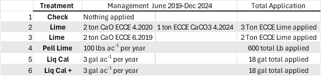
This was a laboratory incubation study. The objective was to evaluation the impact of the liquid Ca product (LiqCa**) on the soil pH, buffer capacity, Ca content and CEC of two acidic soils. LiqCa was applied at three rates to 500 g of soil. The three rates were equivalent to 2, 4, and 6 gallon per acre applied on a 6” acre furrow slice of soil. One none treated check and two comparative products were also applied. HydrateLime (CaO) as applied at rate of Ca equivalent to the amount of Ca applied via LiqCa, which was approximately 1.19 pounds of Ca per acre. Also AgLime (CaCO3) was applied at rates equivalent to 1, 2, and 4 ton effective calcium carbonate equivalency (ECCE). The Ag lime used in the study had a measured ECCE of 92%. The two soils selected for both acidic but had differing soil textures and buffering capacities. The first LCB, had an initial soil pH (1:1 H2O) of 5.3 and a texture of silty clay loam and Perkins had a initial pH of 5.8 and is a sandy loam texture. Both soils had been previously collected, dried, ground, and homogenized. In total 10 treatments were tested across two soils with four replications per treatment and soil.
Project protocol, which has been used to determined site specific liming and acidification rates, was to apply the treatments to 500 grams of soil. Then for a period of eight weeks this soil wetted and mixed to a point of 50% field capacity once a week then allowed to airdry and be mixed again. At the initiation and every two weeks after soil pH was recorded from each treatment. The expectation is that soil pH levels will change as the liming products are impacting the system and at some point, the pH reaches equilibrium and no longer changes. In this soil that point was week six however the trail was continued to week eight for confirmation. See Figures 1 and 2.
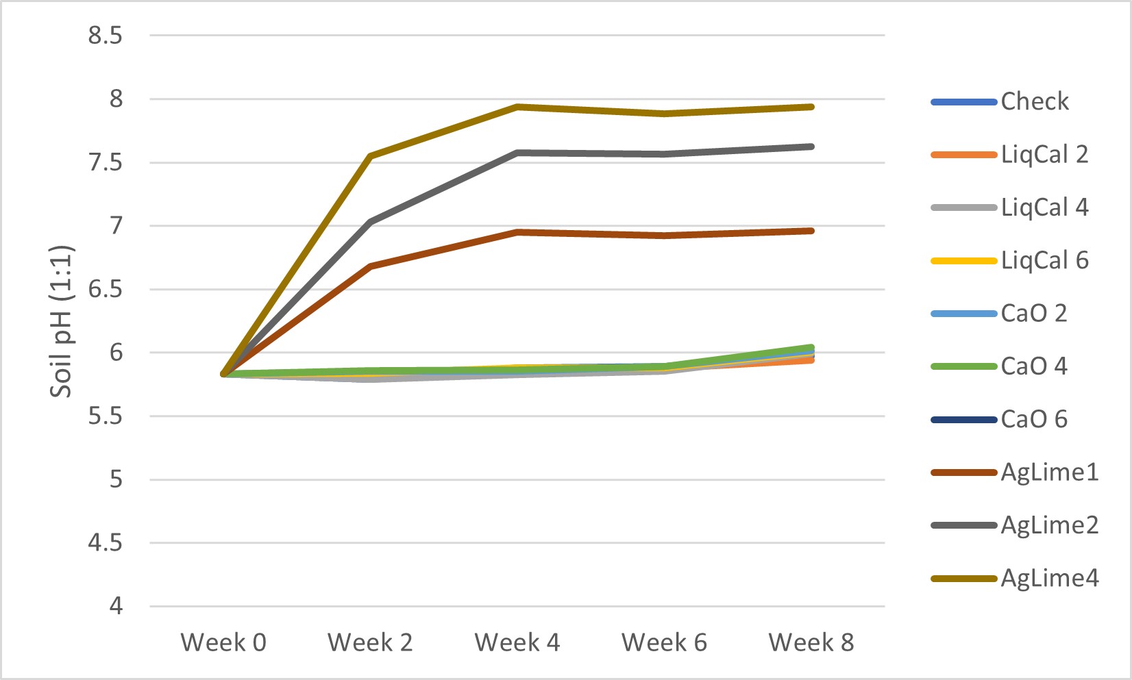
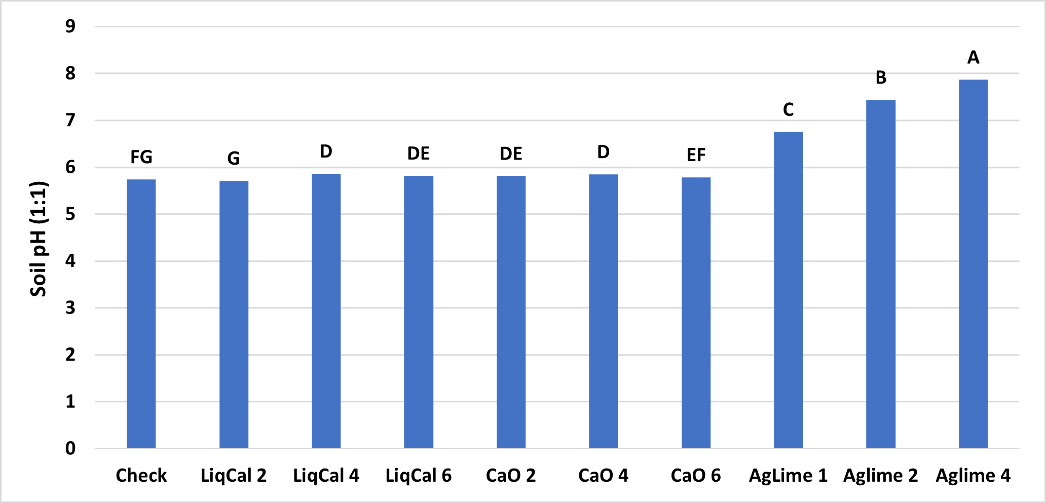
ANOVA Main effect analysis showed that Soil was not a significant effect so therefore both soils were combined for further analysis. Figure 3 shows the final soil pH of the treatments with letters above bars representing significance between treatments. In this study all treatments were significantly greater than the check with exception of LiqCal 2 and CaO 6. Neither LiqCal or CaO treatments reached the pH level of Aglime, regardless of rate.


Summary
The incubation study showed that application of LiqCal at a rate of 4 and 6 gallons per acre did significantly increase the soil pH by 0.1 pH units and 6 gallons per acre increased the Buffer index above the check by 0.03 units. Showing the application of LiqCal did impact the soil. However the application of 1 ton of Ag lime resulted in significantly great increase in soil pH, 1.0 units by 8 weeks and a buffer index change of 0.2 units. The Aglime 1 was statistically greatly than all LiqCal treatments. Ag lime 2 and 4 were both statistically greater than Ag lime 1 with increasing N rate with increasing lime rate. Given the active ingredient listed in LiqCal is CaCl, this result is not unexpected. Ag lime changes pH by the function of CO3 reacting H+ in large quantities. In a unsupported effort a titration was performed on LiqCal, which show the solution was buffered against pH change. However it was estimated that a application of approximately 500 gallons per acre would be needed to sufficiently change the soil pH within a 0-6” zone of soil.
Results of the field study.
https://osunpk.com/2025/06/02/field-evaluation-of-lime-and-calcium-sources-impact-on-acidity/
Take Home
The application of a liquid calcium will add both calcium and chloride which are plant essential nutrients and can be deficient. In a soil or environment suffering from Cl deficiency specifically I would expect an agronomic response. However this study suggest there is no benefit to soil acidity or CEC with the application rates utilized (2, 4, and 6 gallon per acre).
** LiqCal The product evaluated was derived from calcium chloride. It should be noted that since the completion of the study this specific product used has changed its formulation to a calcium chelate. This change however would not be expected to change the results as the experiment did include a equivalent calcium rate of calcium oxide.
Other articles of Interest
https://extension.psu.edu/beware-of-liquid-calcium-products
https://foragefax.tamu.edu/liquid-calcium-a-substitute-for-what/
Any questions or comments feel free to contact me. b.arnall@okstate.edu
Field evaluation of lime and calcium sources impact on Acidity.
At the same time we initiated a lab study looking at the application of LiqCal https://osunpk.com/?p=2096 , we also initiated a field trial to look at the multi-year application of LiqCal, Pelletized Lime and Ag-Lime.
A field study was implemented on a bermudagrass hay meadow near Stillwater in the summer of 2019. The study looked to evaluate the impact of multiple liming / calcium sources impact on forage yield and soil properties. This report will focus on the impact of treatments on soil properties while a later report will discuss the forage results.
Table 1. has the management of the six treatments we evaluated, all plots had 30 gallons of 28-0-0 streamed on each spring in May. Treatment 1 was the un-treated check. Treatment 2, was meant to be a 2 ton ECCE (Effective Calcium Carbonate Equivalency) Ag Lime application when we first implemented the plots in 2019, but we could not source any in time so we applied 2.0 ton ECCE hydrated lime (CaO) the next spring. The spring 2023 soil samples showed the pH to have fallen below 5.8 so and Ag lime was sourced from a local quarry and 1.0 ton ECCE was applied May 2024. Treatment 3, was meant to complement Treatment 2 as an additional lime source of hydrated lime, it was applied June 2019. My project has used hydrated lime as a source for many years as it is fast acting and works great for research. Treatment 4 had 100 lbs. of pelletized lime applied each spring. The 100 lbs. rate was based upon recommendation from a local group that sells Pell lime. Treatments 5 and 6 were two liquid calcium products *Liq Cal * and **Lig Cal+ from the same company. The difference based upon information shared by the company was the addition of humic acid in the Liq Cal+ product. Both LiqCal and LiqCal+ where applied at a rate of 3 gallons per acre per year, with 17 gallons per acre of water as a carrier. Table 1, also shows total application over the six years of the study.
After six years of applications and harvest it was decided to terminate the study. The forage results were intriguing however little differences where seen in total harvest over the six years, highlighting a scenario I have encountered in the past on older stands of bermuda. That data will be shared in a separate blog.
The soils data however showed exceptionally consistent results.
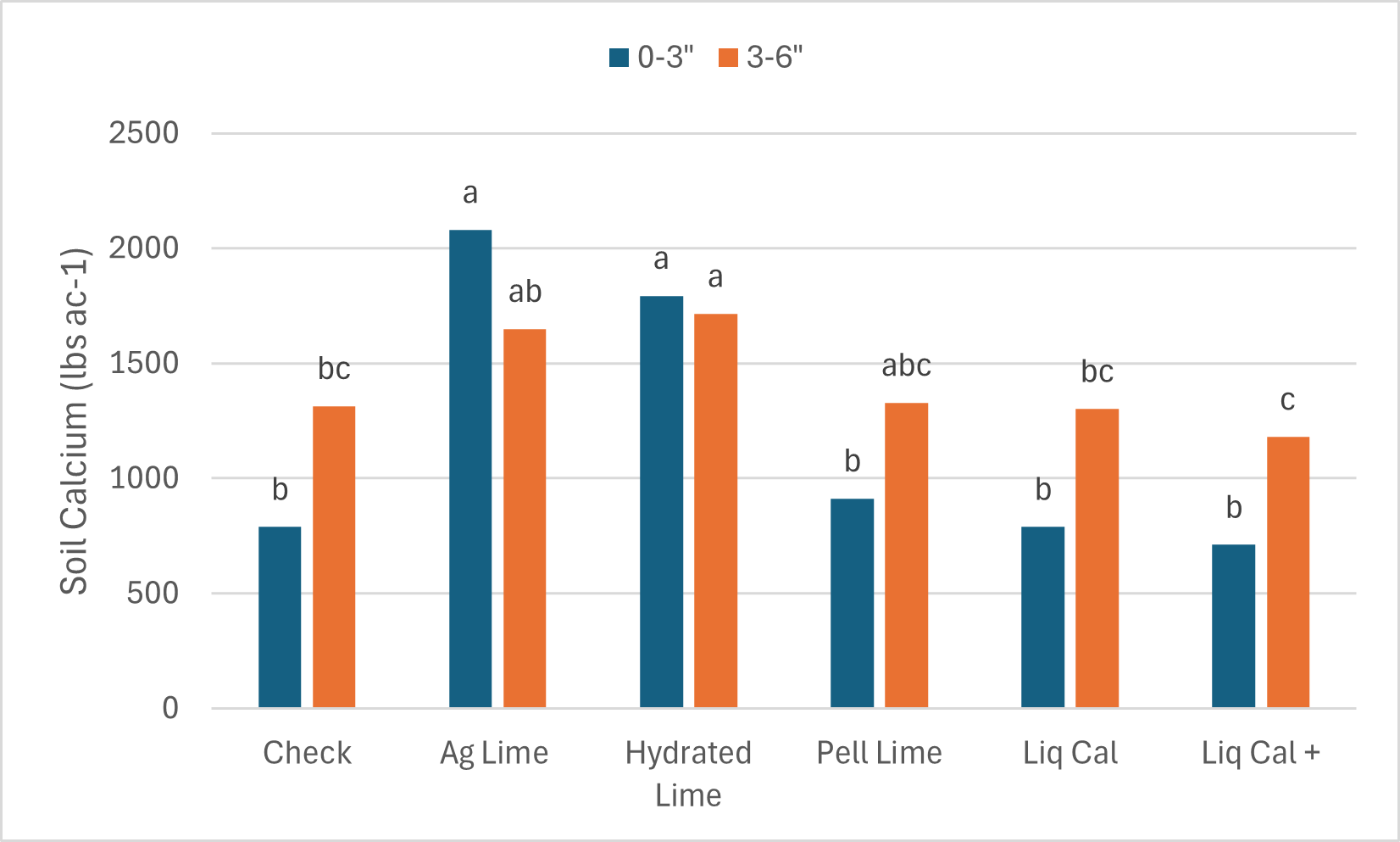
In February of 2025 soil samples were collected from each plot at depths of 0-3 inch’s and 0-6 inches (Table 2.). It was our interest to see if the soil was being impacted below the zone we would expect lime and calcium to move without tillage, which if 0-3″. Figure 1. below shows the soil pH of the treatments at each depth. In the surface (blue) the Ag Lime and Hydrated lime treatments both significantly increased from 4.78 to 6.13 and 5.7 respectively. While the Pel lime, LiqCal and LiqCal+ had statistically similar pH’s as the check at 4.8, 4.65, and 4.65. It is important to note that the Ag Lime applied in May of 2024 resulted in a significant increase in pH from the 2019 application of Treatment 3. The Spring of 2024 soil samples showed that the two treatments ( 2 and 3 ) were equivalent. So within one year of application the Ag lime significantly raised soil pH.
As expected the impact on the 3-6″ soil pH was less than the surface. However, the Ag Lime and Hydrated lime treatments significantly increased the pH by approximately 0.50 pH units. This is important data as the majority of the literature suggestion limited impact of lime on the soil below the 3″ depth.

The buffer pH of a soil is used to determine the amount of lime needed to change the soils pH. In Figure 2. while numeric differences can be seen, no treatment statistically impacted the buffer pH at any soil depth.

The soil calcium level was also measured. As with 0-3″ pH and Buffer pH the Ag Lime and Hydrated lime had the greatest change from the check. These treatments were not statistically greater than the Pell Lime but where higher than the LiqCal and LiqCal+.

Each value is the average of four replicates.
Take Homes
In terms of changing the soils pH or calcium concentration, as explained in the blog https://osunpk.com/2023/01/24/mechanics-of-soil-fertility-the-hows-and-whys-of-the-things/, it takes a significant addition of cations and oxygens to have an impact. This data shows that after six years of continued application of pelletized lime and two liquid calcium products the soil pH did not change. While the application of 2 ton ECCE hydrate lime did.
Also within one year of application Ag lime the soil pH significantly increased.
* LiqCal The product evaluated was derived from calcium chloride. It should be noted that since the completion of the study this specific product used has changed its formulation to a calcium chelate. This change however would not be expected to change the results as the experiment did include a equivalent calcium rate of calcium oxide.
** LiqCal+ The product evaluated was derived from calcium chloride. It should be noted that since the completion of the study this specific product used has changed its formulation. The base was changed from calcium chloride to a calcium chelate. Neither existing label showed Humic Acid as a additive, however the new label has a a list of nutrients at or below 0.02% (Mg, Zn, S, Mn, Cu, B, Fe) and Na at .032% and is advertised as having microbial enhancements.
Any questions or comments feel free to contact me. b.arnall@okstate.edu
Sorghum Nitrogen Timing
Contributors:
Josh Lofton, Cropping Systems Specialist
Brian Arnall, Precision Nutrient Specialist
This blog will bring in a three recent sorghum projects which will tie directly into past work highlighted the blogs https://osunpk.com/2022/04/07/can-grain-sorghum-wait-on-nitrogen-one-more-year-of-data/ and https://osunpk.com/2022/04/08/in-season-n-application-methods-for-sorghum/
Sorghum N management can be challenging. This is especially true as growers evaluate the input cost and associated return on investment expected for every input. Recent work at Oklahoma State University has highlighted that N applications in grain sorghum can be delayed by up to 30 days following emergence without significant yield declines. While this information is highly valuable, trials can only be run on certain environmental conditions. Changes in these conditions could alter the results enough to impact the effect delay N could have on the crop. Therefore, evaluating the physiological and phenotypic response of these delayed applications, especially with varied other agronomic management would be warranted.
One of the biggest agronomic management sorghum growers face yearly is planting rate. Growers typically increase the seeding rate in systems where specific resources, especially water, will not limit yield. At the same time, dryland growers across Oklahoma often decrease seeding rates by a large margin if adverse conditions are expected. If seeding rates are lowered in these conditions and resources are plentiful, sorghum often will develop tillers to overcome lower populations. However, if N is delayed, there is a potential that not enough resources will be available to develop these tillers, which could decrease yields.
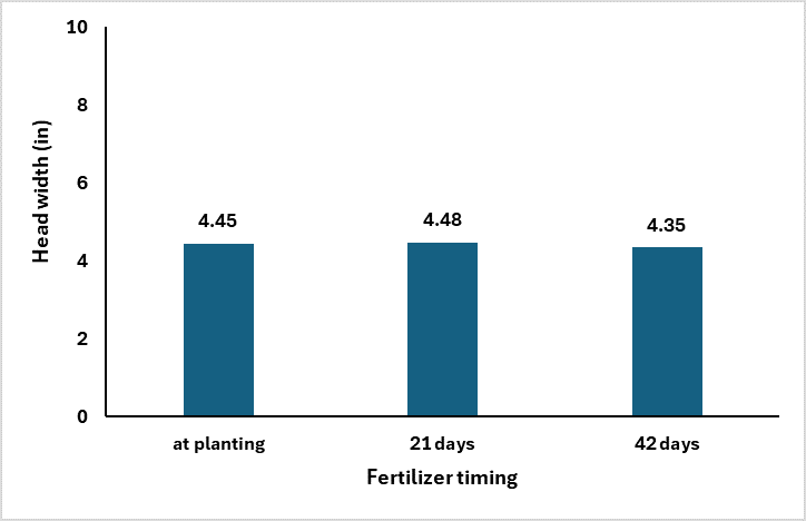
A recent set of trials, summarized below, shows that as N is delayed, the number of tillers significantly decreases over time. Furthermore, the plant cannot overcompensate for the lower number of productive heads with significantly greater head size or grain weight.
This information shows that delaying sorghum N applications can still be a viable strategy as growers evaluate their crop’s potential and possible returns. However, delayed N applications will often result in a lower number of tillers without compensating with increased primary head size or grain weight.
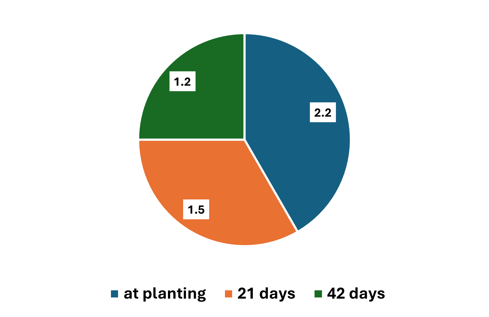

This date on yield components is really interesting when you then consider the grain yield data. The study, which is where the above yield component data came from, was looking at population by N timing. The Cropping Systems team planted 60K seeds per acre and hand thinned the stands down to 28 K (low) and 36K (high). The N was applied at planting, 21 days after emergence, and 42 days after emergence. The rate of N applied was 75 lbs N ac. It should be noted both locations were responsive to N fertilizer.

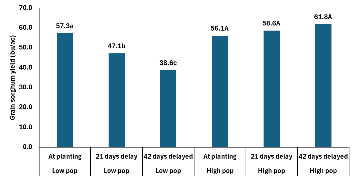
In the data you can without question see how the delayed N management is not a tool for any of members of the Low Pop Mafia. However those at what is closer to mid 30K+ there is no yield penalty and maybe a yield boost with delayed N. The extra yield is coming from the slightly heavier berries and getting more berries per head. Which is similar to what we are seeing in winter wheat. Delaying N in wheat is resulting in fewer tillers at harvest, but more berries per head with slightly heavier berries.
Now we can throw even more data into the pot from the Precision Nutrient Management Teams 2024 trials. The first trial below is a rate, time and source project where the primary source was urea applied in front of the planter for pre in range of rates from 0-180 in 30 lbs increments. Also applied pre was 90 lbs N as Super U. Then at 30 days after planted we applied 90 lbs N as urea, SuperU, UAN, and UAN + Anvol.
Pre-plant urea topped out at 150 lbs of Pre-plant (57 bushel), but it was statistically equal to 90 lbs N 51 bushel. The use of SuperU pre did not statistically increase yield but hit 56 bushel. The in-season shots of 90 lbs of UAN, statistically outperformed 90 pre and hit our highest yeilds of 63 and 62 bushel per acre. The dry sources in-season either equaled their in preplant counter parts.

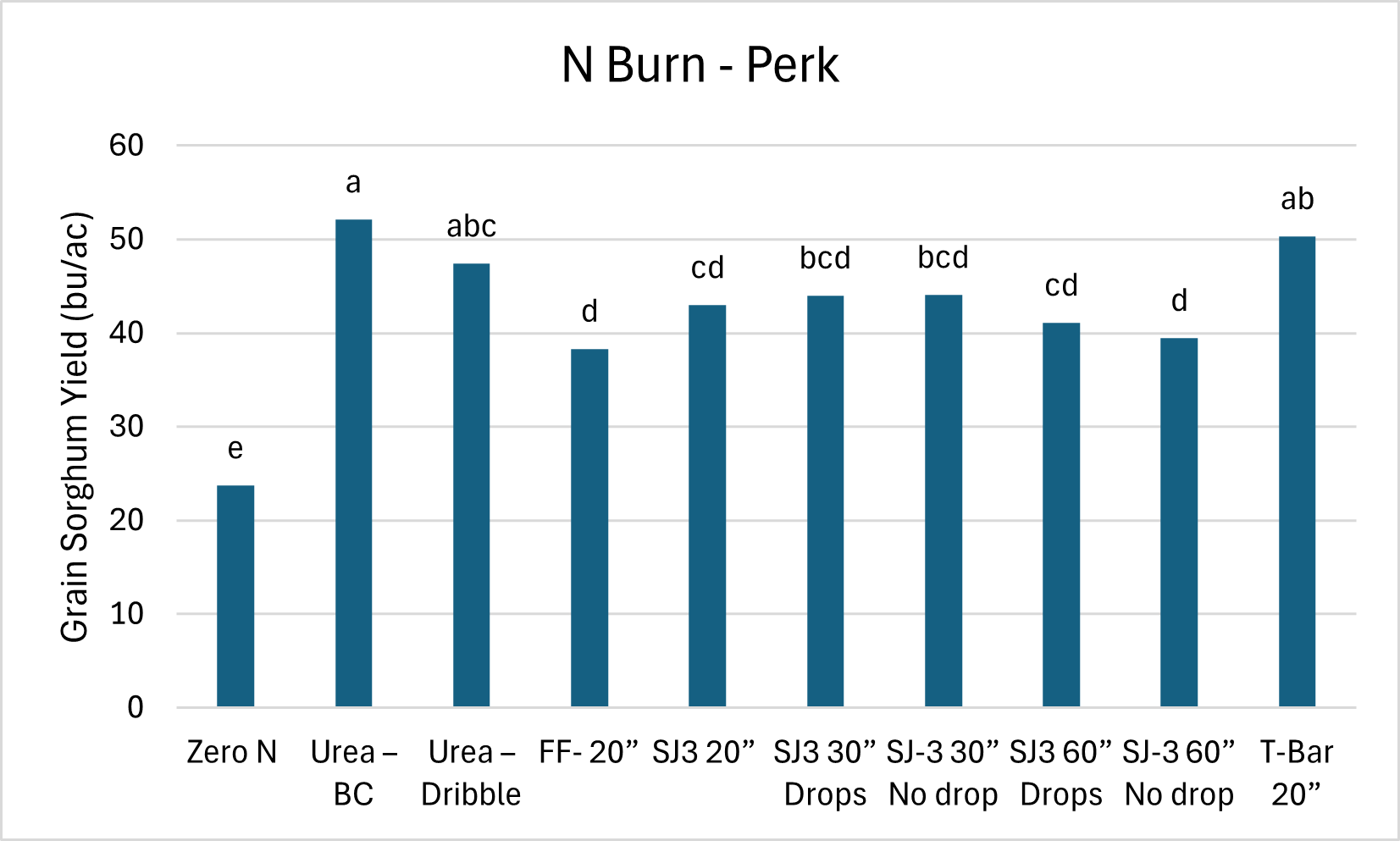
The Burn Study at Perkins, showed that the N could be applied in-season through a range of methods, and still result good yields. In this study 90 lbs of N was used and applied in a range of methods. The treatments for this study was applied on a different day than the N source. Which you can see in this case the dry untreated urea did quite well when when applied over the top of sorghum. In this case we are able to get a rain in just two days. So we did get good tissue burn but quick incorporation with limited volatilization.
Take Home:
Unless working in low population scenarios. The data show that we should not be getting into any rush with sorghum and can wait until we know we have a good stand. We also have several options in terms of nitrogen sources and method of application.
Any questions or comments feel free to contact Dr. Lofton or myself
josh.lofton@okstate.edu
b.arnall@okstate.edu
Funding Provided by The Oklahoma Fertilizer Checkoff, The Oklahoma Sorghum Commission, and the National Sorghum Growers.
Boosting Wheat Grain Protein: Smart Spray Strategies for Better Grain Quality
Brian Arnall, Precision Nutrient Management Specialist
Samson Abiola, PNM Ph.D. Student.
Wheat Protein and Technology challenge
For wheat growers, achieving both high yields and good protein content is a constant challenge. Wheat contributes about 20% of the world’s calories, making it a vital crop for global nutrition. Every season, we face the question of how to boost grain protein concentration (GPC) without sacrificing the yield.
Traditional approaches often involve applying more nitrogen (N) early in the season. While this can help, it is often wasteful, environmentally problematic, and does not always translate to higher protein levels at harvest. The effectiveness of N applications depends not just on timing but also on the spray technology used, including the N source, nozzle type, and droplet size. While protein premiums are never guaranteed, we wanted to develop recommendations prior to the need.
The Research Approach: Timing and Technology
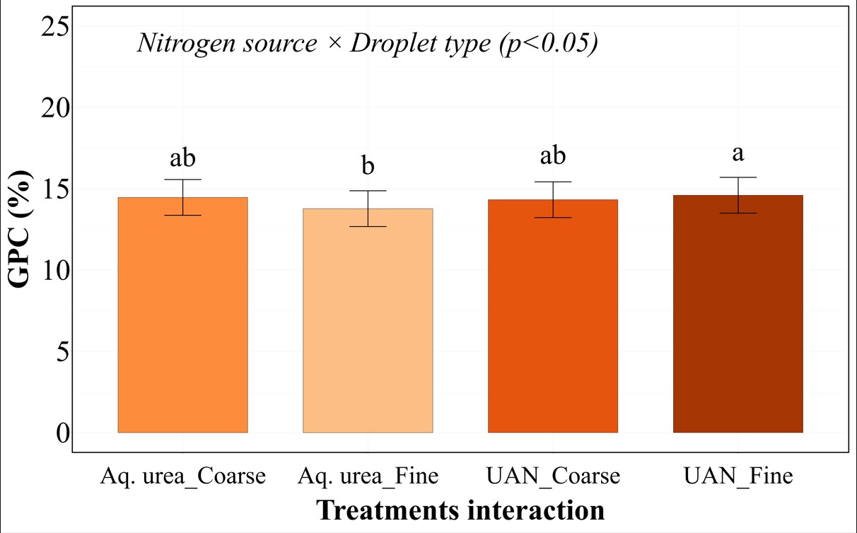
Our research team conducted a comprehensive three-year study (2019-2022) across three Oklahoma locations (Perkins, Lake Carl Blackwell, and Chickasha) to investigate how different combinations of N sources, nozzle types, and droplet sizes affect protein when applied during flowering. We considered two N sources (urea-ammonium nitrate (UAN) and aqueous urea [Aq. Urea]). We also evaluated three nozzle types: Standard flat fan (FF) nozzles with a traditional 110° spray angle, 3D nozzles with three-dimensional spray patterns that enhance canopy penetration, Twin (TW) nozzles with dual forward and rear facing sprays (30° forward and backward)
Finally, we tested both fine droplets (below 141 microns) and coarse droplets (≥141 microns). All applications were made at flowering i.e., when you start seeing yellow anthers sticking out of the wheat heads. Both UAN and Aq. urea were applied at a 20 gpa application rate with a 1:1 dilution with water delivering approximately 30 lbs. of N per acre.
What We Found: More Protein Without Hurting Yield
The big news? Spraying N at flowering boosted wheat protein by 12% without sacrificing yield. This held true across fields yielding anywhere from 30 to 86 bushels per acre. Why doesn’t it hurt yield? By flowering time, your wheat has already “decided” how many heads and kernels it will produce. The N you spray at this stage goes straight to building protein in those existing kernels.
One important caution: Mother Nature still calls the shots, so keep an eye on the forecast before planning your application. If the weather is hot and dry, this is not a good idea. First, those environments typically result in higher protein anyways. But low humidity will significantly increase the likelihood of burn.
Lake Carl Blackwell Findings: UAN Takes the Lead
At our Lake Carl Blackwell site, we saw our highest protein levels reaching up to 16.3% in some plots. In 2020-21, UAN clearly beat Aq. urea (14.7% vs. 14.0% protein). Both were much better than not applying any N at flowering (13.1%) (Figure 1A). Also, the 3D nozzle gave us the highest protein (14.7%), outperforming the control but performing similarly to FF (14.0%) and TW nozzles (14.2% (Figure 1B). The next year (2021-22) showed us something interesting, the combination of N source and droplet size really matters. UAN with fine droplets hit 14.6% protein, similar to UAN with coarse droplets (14.4%) and Aq. urea with coarse droplets (14.3%), but Aq. urea with fine droplets fell behind at just 13.8% (Figure 1C).

Chickasha Results: Matching Your N to the Right Droplet Size
At Chickasha, protein ranged from 10.1% to 13.8% across the two years we studied. In 2021-22, UAN beat Aq. urea (12.7% vs. 12.2%), and both beat the control (11.8%) (Figure 2A). Also, the 3D nozzle (12.8%) outperformed both FF and TW nozzles (both 12.2%) (Figure 2B).
In 2020-21, we found that the combination of N source, nozzle type, and droplet size all worked together to affect protein. The winning combination was UAN with 3D nozzle and fine droplets (13.23% protein), which performed similarly to Aq. urea with TW nozzle and coarse droplets (13.18%) (Figure 2C). The least performer was Aq. urea with TW nozzles and fine droplets (12.20%) among the treatments. This shows how weather and growing conditions can change which factors matter most from year to year
Perkins Results: Getting Every Detail Right
At our Perkins site, we saw protein levels ranging from 10% to 13.1%. Here, the combination of all three factors (N source, nozzle type, and droplet size) made a huge difference. The best setup was UAN with 3D nozzle and coarse droplets (12.2% protein). The worst was Aq. urea with TW nozzle and fine droplets (10.5%) (Figure 3). That’s a 15% difference that could mean the difference between premium and feed-grade wheat!
UAN consistently outperformed Aq. Urea across all setups. For example, UAN with 3D nozzle and coarse droplets produced 10% higher protein than the same setup with Aq. Urea.

Equipment and Application Recommendations
Over the three years UAN consistently outperformed perform Aq. urea, showing there is no need for a special formulation and that commercially available UAN is all we really need as a source. While no nozzle type significantly stood out across all sites the 3-D nozzle did show up a couple times as being statistically better. So the important message would be that while the high tech nozzles could provide some value the traditional flat fan performed quite well. While some differences were seen in droplet size, the lack of consistency leads us to say focus on good coverage with limited drift.
Take-Home Messages
- Foliar N at flowering boosted wheat protein by 12% without affecting yield multiple growing seasons and locations. This increase was from 0.5 to nearly 2.0 % protein.
- Nitrogen source matters – UAN consistently outperformed Aq. Urea.
- Your spray technology mattered but not lot – and 3D nozzles generally gave the best results. The good ole flat fans nozzles still did quite will.
- Match droplet size to your setup – generally fine for UAN and coarse for Aq. Urea.
- This targeted approach enhances grain quality without sacrificing yield, potentially improving grain prices and profitability while using N more efficiently.
- Mother Nature still calls the shots, so keep an eye on the forecast before planning your application. If the weather is hot and dry, this is not a good idea. First, those environments typically result in higher protein anyways. But low humidity will significantly increase the likelihood of burn.
This blog was written based upon the data published in the manuscript “Optimizing Spray Technology and Nitrogen Sources for Wheat Grain Protein Enhancement” which is available for free reading and downloading at https://www.mdpi.com/2077-0472/15/8/812
Any questions or comments feel free to contact me. b.arnall@okstate.edu
Nitrogen and Sulfur in Wheat
Brian Arnall, Precision Nutrient Management Specialist
Samson Abiola, PNM Ph.D. Student.
Nitrogen timing in wheat production is not a new topic on this blog, in-fact its the majority. But not often do we dive into the application of sulfur. And as it is top-dressing season I thought it would be a great opportunity to look at summary of a project I have been running since the fall of 2017 which the team has call the Protein Progression Study. The objective was to evaluate the impact of N and S application timings on winter wheat grain yield and protein. With a goal of looking at the ratio of the N split along with the addition of S and late season N and S, in such a way that we could determine BMP for maximizing grain yield and protein.
My work in the past has shown two things consistently, that spring N is better on the average and S responses have been limited to deep sandy soils in wet years. Way back when (2013) on farm response strips showed high residual N at depth and no response to S. https://osunpk.com/2013/06/28/response-to-npks-strips-across-oklahoma/. But there has been a lot of grain grown since that time expectations are that we should/are seeing an increase in S response. In fact Kansas State is seeing more S response, especially in the well drained soils in east half of the state.
Some KSU Sulfur works.
https://www.ksre.k-state.edu/news/stories/2022/04/video-sulfur-deficiency-in-wheat.html
https://eupdate.agronomy.ksu.edu/article/sulfur-deficiency-in-wheat-364-1
Click to access sulphur-in-kansas-plant-soil-and-fertilizer-considerations_MF2264.pdf
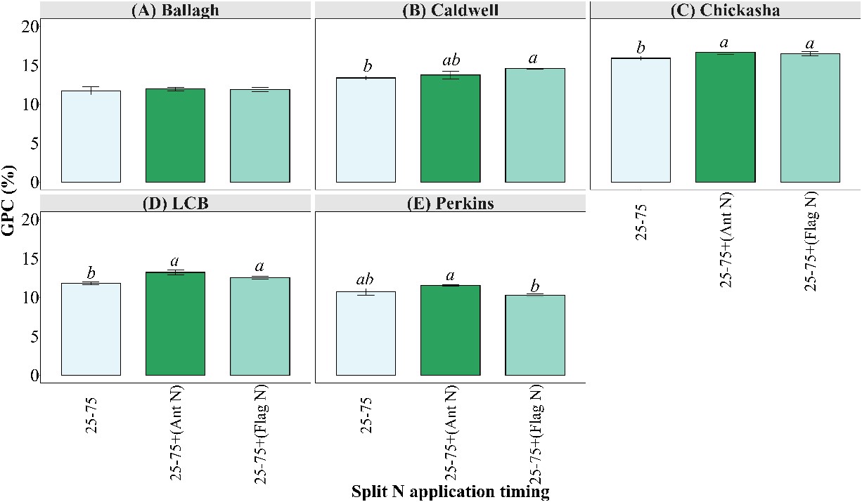
So the Protein Progression Project was established in 2017 and where ever we had space we would drop in the study. So in the end across six seasons we had 13 trials spread over five locations. Site-years varied by location: Chickasha (2018-2022), Lake Carl Blackwell (2018-2023), Ballagh (2020), Perkins (2021), and Caldwell (2021).

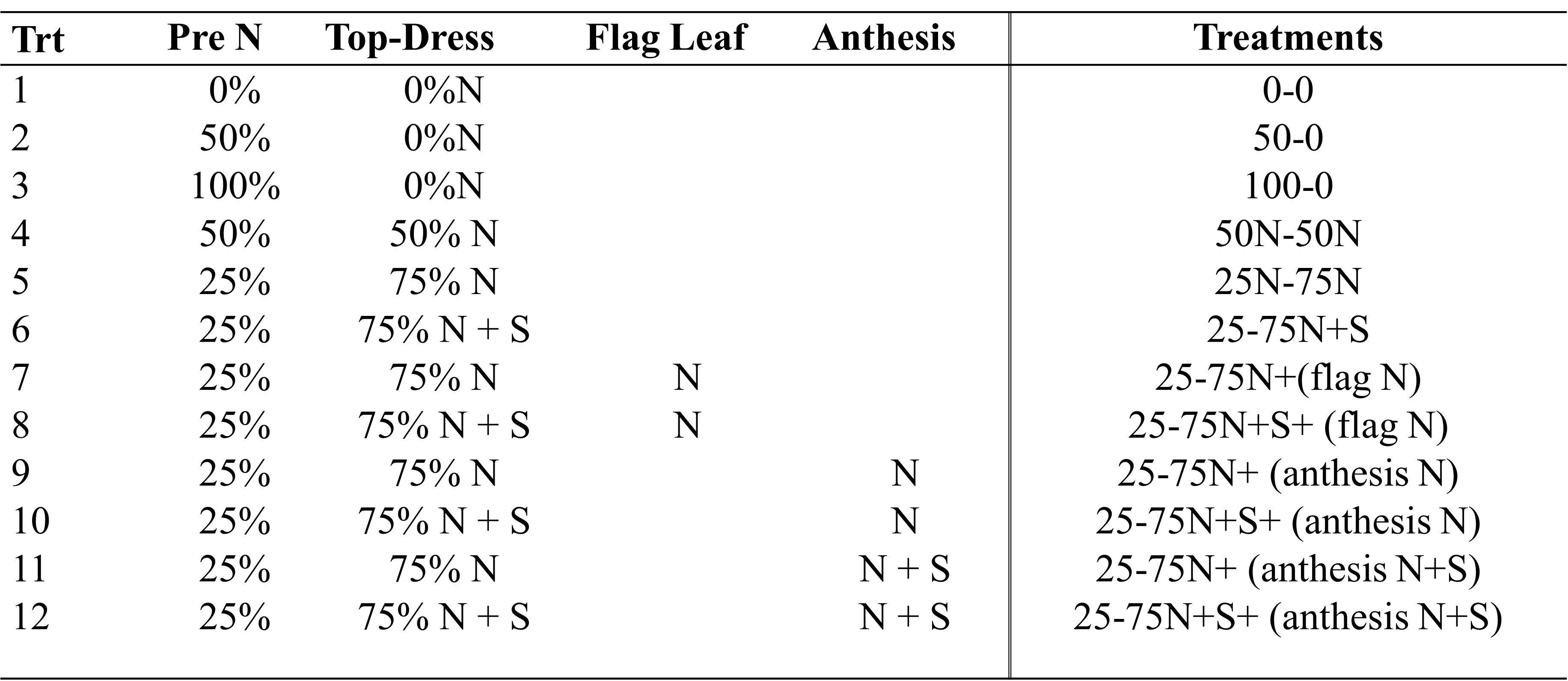
First lets just dive into the the N application were we looked at 100% pre vs 50-50 split and 25-75 split (Table 2.) Based upon the wealth of previous work https://osunpk.com/2022/08/26/impact-of-nitrogen-timing-2021-22-version/, its not much of a surprise that split application out preformed preplant and that having the majority applied in-season tended to better grain yields and protein values.

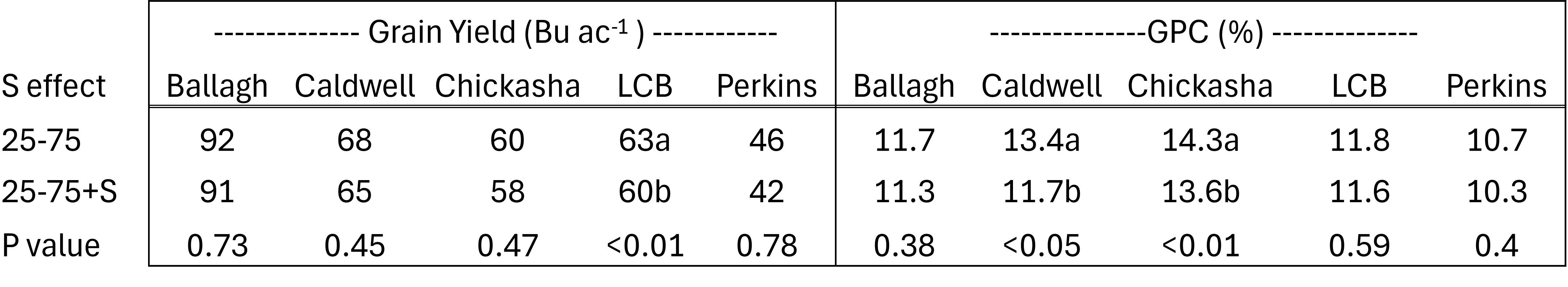
This next table is were things get to be un-expected. While the data below is presented by location, we did run each site year by itself. In no one site year did S statistically, or numerically increase yield. As you can see in Table 2 below, the only statistical response was a negative yield response to S. And you can not ignore the trend that numerically, adding S had consistently lower yields. Even more surprising was the same trend was seen in Protein.
One aspect of Protein Progression trials were that while 0-6″ soil test S tended to be low. We would often find pretty high levels of S when we sampled deeper, especially when there was a clay increase with depth. Sulfur tends to be held by the clay in our subsoil. We are also looking at better understanding the relationship between N and S. In fact a review article published in 2010 discussed that the N and S ratio can negative influence crop production when either one of the elements becomes un-balanced. For example we are seeing more often in corn that when N is over applied we can experience yield loss, unless we apply S. Meaning at 200 lbs of N we make 275 BPA, at 300 N lbs we make 250, but 300 N plus 20 S we can make 275 again. Part of the rationale is that excessive N limits S mineralization. On the flip side if S is applied while N is deficient and yield decrease could be experienced. Maybe that is what we are seeing in this date. Either way, this data is why the Precision Nutrient Management program is spending a fair amount of efforts in understanding the N x S relationship in wheat (which we are looking at milling quality also) and corn.
A quick dive into increasing protein with late N applications. At three of the five location GPC was significantly increased with Late N. In most cases the anthesis (flowering) application was the highest with exception of Caldwell. We will have another blog coming out in a month that digs into anthesis applied N at a much deeper level, looking at source, nozzle and droplet sizes.
Looking at this study in a vacuum we can say that it probably best to split apply your N and that in central and northern Ok the addition of S in rainfed wheat doesn’t offer great ROI. If I look at the whole picture of all my work and experience I would offer this. For grain only wheat, the majority if not all N should be applied in-season sometime between green up and two weeks after hollow stem. I have had positive yield responses to S applied top-dress, but it has always been deep sandy soils and wet seasons. I have not have much is any response to S in heavier soil, especially if there is a clay increase in the two feet of profile. So my general S recommendation is 10 lbs in sandy soils and if you show low soil test S in heavier ground and you are trying to push grain yields, then you could consider the addition of S as a potential insurance. That said, I haven’t seen much proof of it.
Take Homes
* Split application of nitrogen resulted in higher grain yields and protein concentrations when compared to 100% preplant.
* Putting on 75% of the total N in-season tended to result in higher grain yields and protein concentrations when compared to 50-50 split.
* Adding 10 lbs of S topdress did not result in any increase in grain yield or protein.
A big Thanks to the collaborators providing on-farm locations for this project. Ballagh Family Farms, Turek Family Farms and Tyler Knight.
Citation. Jamal, A.,*, Y. Moon, M. Abdin. 2010 Review article. Sulphur -a general overview and interaction with nitrogen. AJCS 4(7):523-529 (2010). ISSN:1835-2707.
Any questions or comments feel free to contact me. b.arnall@okstate.edu
