
The Mechanics of Soil Fertility: Use of Sugar in Field Crops
Jolee Derrick, Precision Nutrient Management Ph. D. Student
Grace Williams, Soil Microbiology Ph. D. Candidate
Brian Arnall, Precision Nutrient Management Specialist
Recently, there has been increased interest in adding sugar to spray tank mixes, whether for post-emergence weed control or foliar nutrient applications. While there is limited work on impact of sugar inclusion in herbicide applications, some papers have posed potential enhancement (Devine and Hall, 1990). But since this is coming from a soil science group, we will only focus on soil impact. Following up the last blog, unlike humic substances, which represent more complex and relatively stable carbon forms, sugar is a highly labile carbon source. This rapid utilization of simple carbon sources is well documented to stimulate microbial activity and growth (Kuzyakov and Blagodatskaya, 2015). The general idea of utilizing sugar applications is that sugar has the capacity to improve spray performance, stimulate biological activity, increase organic matter mineralization, and ultimately result in improved yields.
Sugar additions can influence soil processes differently depending on system conditions. In systems with higher residual nitrogen and organic matter, responses may differ from those observed in Oklahoma production environments, where soils are typically lower in organic matter and microbial activity can occur for much of the year. Understanding how sugar functions in these systems requires a basic discussion of carbon dynamics. Sugar itself is almost entirely carbon and is readily consumed by microbes. It’s a simple molecule, which allows it to dissolve easily in water and be quickly utilized in the soil system. Crop residues, like wheat straw, are also carbon-rich but much more complex. They contain cellulose, hemicellulose, and lignin which are long carbon chains that take time to break down because microbes need specialized enzymes to access them.
For the sake of simplicity, we can group carbon into two key pools: labile carbon and particulate organic matter (POM). Labile carbon includes easily decomposed materials, which include the previously mentioned simple sugars that microbes can metabolize rapidly. These pools differ in turnover time and microbial accessibility, with labile carbon driving short-term microbial responses (Cotrufo et al. 2013). POM breaks down more slowly and serves as a longer-term nitrogen source through residue breakdown.
Soil microorganisms require both carbon and nitrogen to grow and maintain biomass, typically at a ratio of approximately 24 parts carbon to 1 part nitrogen. When readily available carbon is abundant, but nitrogen is limited, microbes increase their nitrogen demand and begin scavenging nitrogen from the surrounding soil. This process, better known as nitrogen immobilization, temporarily reduces nitrogen availability to crops. Additions of readily available carbon sources have consistently been shown to increase microbial nitrogen immobilization in soil systems (Recous et al. 1990).
In systems where sufficient nitrogen is present, microbial populations can expand rapidly. Fast-growing microbial species may dominate, continuing to immobilize nitrogen within their biomass. Eventually, when nitrogen becomes limiting, microbial populations decline to levels the system can support. This boom-and-bust cycle can disrupt nitrogen availability during critical stages of crop growth. These rapid shifts in microbial population and activity following carbon inputs are commonly observed in soil systems receiving easily decomposable substrates (Blagodatskaya and Kuzyakov, 2008).
This dynamic becomes especially relevant when considering residue management practices common in Oklahoma. Under no-till or limited-tillage systems, the crop residues have wide carbon-to-nitrogen (C:N) ratios, creating conditions where nitrogen immobilization can occur during the growing season.
Table 1 provides approximate C:N ratios for several crops commonly grown in Oklahoma. When additional carbon is introduced into these systems without accompanying nitrogen, the likelihood of microbial immobilization increases. While immobilization is not bad, it does create a question mark as Oklahoma’s variable climate means the following release of nutrients will be unpredictable.
Table 1. Table depicting the range of C:N ratios for residues of commonly utilized crops in Oklahoma. Ratios were obtained from Brady, N. C., & Weil, R. R. (2017). The Nature and Properties of Soils (15th ed.)

Now consider conventional tillage systems. In Oklahoma, no-till systems typically contain 2 to 3 percent organic matter, which is relatively high given our climate and extended periods of microbial activity. Conventional tillage systems often fall between 0.75 and 2.25 percent organic matter. Because soil organic matter is approximately 58 percent carbon, this represents a substantial difference in the soil carbon pool.
Tillage can temporarily enhance microbial access to both previously mentioned carbon pools. When tillage exposes previously protected carbon, microbial activity increases rapidly. This initial flush can temporarily increase nitrogen mineralization as organic nitrogen is converted to plant-available forms. However, this phase is short-lived. As microbial populations expand, nitrogen demand increases, leading to immobilization and reduced nitrogen availability.
Hypothetically, increased microbial growth and activity would rapidly mineralize organic matter, trigger a surge in NO₃⁻, deplete soil organic matter, and as resources become limiting and the environment can no longer sustain elevated microbial populations, this boom would be followed by a population crash. This relationship is ultimately driven by the soil C:N ratio, which introduces an interesting additional complexity of residue. Different residues bring very different carbon-to-nitrogen balances into the system, and microbes respond accordingly. High carbon residues give microbes plenty of energy but very little nitrogen, so they pull N out of the soil to meet their needs. Residues with lower C:N ratios (soybean, alfalfa, etc.) do opposite, releasing nitrogen as they break down. Now the real question becomes where the critical point sits, and when does management push the system from the threshold of immobilization and mineralization.
These hypotheses form the foundation for new research currently underway through the Precision Nutrient Management Program. Initial proof-of-concept work has already been completed, providing a necessary steppingstone to address these questions.
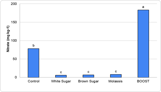
Figure 1. Graph depicting the different concentrations of nitrate leached corresponding to applied treatments in the proof-of-concept work
The preliminary work (Figure 1) evaluated different sugar sources applied alongside a high-nitrogen product to assess the extent of nitrogen immobilization. Although these studies were conducted using potting soils, clear trends were apparent. Treatments containing sugar consistently showed greater nitrogen immobilization compared to treatments without sugar. This response is consistent with studies showing that additions of simple carbon substrates stimulate microbial growth and increase nitrogen immobilization (Dendooven et al. 2006). Building on this work, an active field-based research project is underway to evaluate how sugar additions influence nitrogen availability and microbial dynamics under real-world Oklahoma production conditions.
From an agronomic standpoint, sugar functions primarily as a readily available carbon source that stimulates microbial growth. In nitrogen-limited systems, this response increases the likelihood that nitrogen will be incorporated into microbial biomass rather than remaining immediately available for crop uptake.
Finally, we conclude with a conceptual consideration. If increased OM mineralization leads to greater plant biomass, this process may partially offset losses of OM. Greater biomass production could return more residues to the soil, contributing to the OM pool in the upper soil profile. Therefore, the system may compensate for OM mineralization through the rebuilding of organic matter via plant inputs. However, the stabilization of this carbon depends on microbial processing and physical protection within the soil matrix (Cotrufo et al. 2015)
However, while the underlying logic is sound, this concept has not been extensively studied within Oklahoma cropping systems. This blog does not address the impact of sugar applications on residue breakdown, and the potential impact of such. Future research through the Precision Nutrient Management Program will further investigate the mineralization process to better understand carbon dynamics within these systems.
Take Home:
- Oklahoma production systems generally have lower residual N and high carbon residues, creating conditions conducive to N immobilization
- Adding sugar increases microbial growth, creating population booms that will momentarily increase mineralization, but then immediately immobilize residual nitrogen.
- Tillage can amplify the negative effects of sugar by exposing more carbon and reducing soil organic matter
- Proof-of-concept work shows sugar triggered a net nitrogen immobilization in a carbon heavy environment
- Proof-of-concept work also suggests that when additional nitrogen is present, sugar additions may shift the system toward net mineralization rather than immobilization.
Work Cited:
Blagodatskaya, E., & Kuzyakov, Y. (2008). Mechanisms of real and apparent priming effects. Biology and Fertility of Soils, 45, 115–131.
Brady, N. C., and R. R. Weil. “The Nature and Properties of Soils, 15th Edn (eBook).” (2017).
Cotrufo, M. F., Wallenstein, M. D., Boot, C. M., Denef, K., & Paul, E. (2013). The Microbial Efficiency-Matrix Stabilization (MEMS) framework. Global Change Biology, 19, 988–995.
Cotrufo, M. F., Soong, J. L., Horton, A. J., Campbell, E. E., Haddix, M. L., Wall, D. H., & Parton, W. J. (2015). Formation of soil organic matter via biochemical and physical pathways of litter mass loss. Nature Geoscience, 8(10), 776–779.
Dendooven, L., Verhulst, N., Luna-Guido, M., & Ceballos-Ramírez, J. M. (2006). Dynamics of inorganic nitrogen in nitrate- and glucose-amended alkaline–saline soil. Plant and Soil, 283(1–2), 321–333.
Devine, M. D., & Hall, L. M. (1990). Implications of sucrose transport mechanisms for the translocation of herbicides. Weed Science, 38(3), 299–304.
Kuzyakov, Y., & Blagodatskaya, E. (2015). Microbial hotspots and hot moments in soil: Concept & review. Soil Biology and Biochemistry, 83, 184–199.
Recous, S., Mary, B., & Faurie, G. (1990). Microbial immobilization of ammonium and nitrate in cultivated soils. Soil Biology and Biochemistry, 22, 913–922.
Mechanics of Soil Fertility: Understanding Humic and Fulvic Acids
Brian Arnall, Oklahoma State University, Precision Nutrient Management Extension Specialist
Oliver Li, Oklahoma State University, Soil Chemistry
Interest in humic and fulvic acid products has increased substantially in agricultural production systems during the past two decades. These materials are frequently promoted as tools for improving soil biology, increasing nutrient availability, enhancing fertilizer efficiency, and stimulating plant growth. Because humic substances are known to be important components of soil organic matter, it is reasonable to ask whether adding humic or fulvic products to soil can meaningfully influence soil fertility.
As with many soil fertility questions, the answer depends on understanding two key factors: the mechanism involved and the magnitude of that mechanism relative to the soil system. Soil processes operate within large natural pools of organic matter, nutrients, and microbial activity. Therefore, evaluating the potential effects of humic products requires examining both how these compounds function chemically and biologically and how their application rates compare with the soils organic matter.
What Are Humic and Fulvic Acids?
Humic substances are heterogeneous organic compounds formed during the decomposition and transformation of plant and microbial residues. Historically, soil scientists have divided these materials into three operational fractions based on their solubility behavior: humic acid, fulvic acid, and humin (Stevenson, 1994; Tan, 2014). Humic acids are relatively large molecules that are insoluble under acidic conditions but dissolve in alkaline solutions. Fulvic acids are smaller molecules that remain soluble across the entire pH range, which allows them to move more freely in soil solution.
Both humic and fulvic acids contain numerous functional groups, particularly carboxyl and phenolic groups, which carry negative charge. These functional groups allow humic substances to interact with metal ions and nutrient cations and contribute to several important soil properties, including cation exchange capacity, buffering capacity, and metal complexation (Stevenson, 1994; Lehmann and Kleber, 2015). Because these materials originate from decomposed organic residues, they represent one portion of the complex mixture that collectively makes up soil organic matter. The distribution of the soil organic matter fractions varies among soil types and land uses, but fulvic acids and humic acids are each typically estimated to comprise approximately 10–35% of total soil organic matter (Guimarães et al., 2013).
Nutrient Retention and the Role of Cation Exchange
One of the most commonly cited mechanisms associated with humic substances is their ability to retain nutrients through cation exchange. The negatively charged functional groups present on humic molecules attract positively charged ions in soil solution. Through this electrostatic attraction, humic materials can retain several plant nutrients, including ammonium, potassium, calcium, magnesium, and certain micronutrients such as zinc and copper (Stevenson, 1994; Tan, 2014). This mechanism functions in the same manner as cation exchange on clay minerals. Of course, negatively charged surfaces do not retain negatively charged ions. As a result, nutrients such as nitrate are not held by humic substances and remain mobile in soil solution.
Laboratory measurements indicate that humic materials may possess relatively high cation exchange capacity on a mass basis. Reported values commonly range from approximately 300 to 600 cmolc kg⁻¹ depending on the source material and extraction method (Stevenson, 1994; Tan, 2014). These values demonstrate that humic substances can retain a large amount of cationic nutrients. A question that can be posed, however, is how this capacity compares with the nutrient retention already provided by soil organic matter.
Understanding the magnitude of humic additions requires comparing product application rates with the organic matter already present in soil. Calculations based on typical cation exchange values suggest that one pound of humic material with a CEC of 300–600 cmolc kg⁻¹ could theoretically retain approximately 0.04 to 0.08 pounds of ammonium-nitrogen. When viewed in isolation this number may appear meaningful. However, agricultural soils already contain large quantities of organic matter. An acre furrow slice, representing approximately the upper six inches of soil, weighs roughly two million pounds. Soil containing one percent organic matter therefore contains about 20,000 pounds of organic material per acre (Brady and Weil, 2016). Humified organic matter typically has cation exchange capacities ranging between 150 and 300 cmolc kg⁻¹ (Stevenson, 1994), meaning that the exchange capacity associated with native soil organic matter is already substantial. To put this into perspective, one pound of humic material can retain roughly 0.04 to 0.08 pounds of cation charge. Ammonium and potassium carry a single positive charge, while calcium carries two, meaning two ammoniums can be held for every two calcium. To provide contrast to the application of a humic substance, increasing soil organic matter by just 0.1% equivalent to about 2,000 pounds of additional organic material per acre can provide the capacity to retain approximately 40 to 80 pounds of cation charge or 40 to 80 pounds of ammonium.
The key point is not that humic materials cannot retain nutrients. They clearly can. Rather, the scale of material already present in soil is extremely large compared with the few ounces or pounds of humic products typically applied in agricultural systems. Consequently, the nutrient retention capacity associated with soil organic matter overwhelmingly dominates the soil system.
Micronutrient Complexation
Humic and fulvic substances are also known to interact with micronutrients through metal complexation reactions (also known as ‘chelation’). Carboxyl and phenolic functional groups can coordinate with metal ions such as iron, zinc, copper, and manganese to form organic complexes (Stevenson, 1994; Tan, 2014). These complexes can influence micronutrient mobility and availability in soils.
Fulvic acids are particularly effective at forming soluble complexes because they remain dissolved across the full range of soil pH. In some cases, these complexes may increase micronutrient mobility and transport within the soil solution. This mechanism has been well documented in soil chemistry research and may explain some responses observed in systems where micronutrient availability is limited.
Effects on Plant Physiology
In addition to soil chemical interactions, humic substances may influence plant growth through physiological mechanisms occurring in the rhizosphere. Several studies have shown that humic substances can stimulate root development, including increases in root elongation, lateral root formation, and root hair production (Nardi et al., 2002; Canellas and Olivares, 2014).
Research suggests that these responses may involve interactions with plant hormonal pathways and membrane transport processes. Humic substances have been shown to activate plasma membrane H⁺-ATPase enzymes, which are involved in proton pumping and nutrient uptake across root membranes (Canellas et al., 2002; Trevisan et al., 2010). Activation of these transport systems can enhance nutrient absorption and influence root architecture.
These physiological effects appear to occur primarily at the root–soil interface, where dissolved organic molecules interact directly with plant tissues. As a result, the responses observed in plant growth experiments are often attributed to rhizosphere signaling processes rather than large changes in bulk soil fertility.
Microbial Responses to Humic and Fulvic Compounds
Soil microorganisms respond strongly to carbon availability, and different carbon sources can produce very different microbial responses. Simple carbohydrates such as glucose and sucrose are readily metabolized by soil microbes and therefore produce rapid increases in microbial respiration and biomass. Humic substances, in contrast, consist of chemically complex and partially oxidized organic compounds that decompose much more slowly (Lehmann and Kleber, 2015).
Experimental studies comparing carbon sources consistently show that microbial respiration increases dramatically when simple sugars are added to soil, whereas humic substances produce smaller responses (Blagodatskaya and Kuzyakov, 2008). This difference reflects the relative degradability of these compounds as microbial energy sources.
Carbon Inputs from Humic Products Compared with Natural Soil Carbon
Soil microbial activity is largely driven by carbon supplied from plants through root exudation, residue decomposition, and organic matter turnover. The carbon pools already present in soil are therefore important for understanding the potential influence of humic product additions. A soil containing one percent organic matter holds approximately 11,600 pounds of carbon per acre (Brady and Weil, 2016).
Research on plant–soil carbon cycling indicates that living roots release significant quantities of organic carbon into soil each growing season through root exudation and rhizodeposition (Kuzyakov and Domanski, 2000). These plant-derived carbon inputs commonly amount to hundreds of pounds of carbon per acre and serve as a major energy source for soil microbial communities. Viewed in this context, humic product applications represent extremely small additions to the soil carbon pool. Consequently, microbial stimulation in agricultural soils is dominated by carbon inputs from plant residues and root exudates rather than by small additions of humic materials.
Building Organic Matter in the Central Plains
Increasing soil OM in the central Great Plains is achievable, but the magnitude of change is governed primarily by carbon inputs and water availability rather than any single management practice. Systems that combine no-till, increased residue return, diversified crop rotations, and where feasible cover crops or manure inputs are the most effective because they simultaneously increase carbon inputs and reduce decomposition losses (Lyon et al., 2007; Mikha et al., 2013; Nielsen et al., 2016). In semi-arid systems, realistic rates of OM increase are modest: over a 5-year period, changes are often small, approximately +0.05 to 0.1% OM, but significant in relation to the system which is often at total OM levels between 0.7 and 1.25 prior to establishment of conservation practices. The increase is confined to the top inch of the soil surface (Mikha et al., 2013; Saha et al., 2024). Mechanistically, these gains occur through greater residue and root-derived carbon inputs, reduced soil disturbance which slows microbial oxidation, and improved aggregation that physically protects organic matter from decomposition (Six et al., 2002; Lehmann and Kleber, 2015). However, as emphasized throughout this discussion, the scale of change is small relative to the large existing organic matter pool, and meaningful increases require long-term, system-level management focused on maximizing biomass production rather than relying on small external carbon additions such as commercial products.
Take-Home Points
- Humic and fulvic acids can retain cations, chelate micronutrients, and influence plant and microbial processes.
- Typical application rates are small relative to existing soil organic matter, so whole-soil impacts are limited.
- Most observed effects are localized in the rhizosphere, not broad changes in soil fertility.
- Evaluating both mechanism and scale is key to understanding their role in nutrient management.
References
Blagodatskaya, E., & Kuzyakov, Y. (2008). Mechanisms of real and apparent priming effects and their dependence on soil microbial biomass and community structure. Biology and Fertility of Soils, 45(2), 115–131.
Brady, N. C., & Weil, R. R. (2016). The nature and properties of soils (15th ed.). Pearson.
Canellas, L. P., Olivares, F. L., Okorokova-Façanha, A. L., & Façanha, A. R. (2002). Humic acids isolated from earthworm compost enhance root elongation and lateral root emergence in maize. Plant Physiology, 130(4), 1951–1957.
Canellas, L. P., & Olivares, F. L. (2014). Physiological responses to humic substances as plant growth promoters. Chemical and Biological Technologies in Agriculture, 1, 3.
Guimarães, D. V., Gonzaga, M. I. S., Silva, T. O., Silva, T. L., Dias, N. S., & Matias, M. I. S. (2013). Soil organic matter pools and carbon fractions in soil under different land uses. Soil and Tillage Research, 126, 177–182.
Kuzyakov, Y., & Domanski, G. (2000). Carbon input by plants into the soil: Review. Journal of Plant Nutrition and Soil Science, 163(4), 421–431.
Lehmann, J., & Kleber, M. (2015). The contentious nature of soil organic matter. Nature, 528(7580), 60–68.
Lovley, D. R., Coates, J. D., Blunt-Harris, E. L., Phillips, E. J. P., & Woodward, J. C. (1996). Humic substances as electron acceptors for microbial respiration. Nature, 382, 445–448.
Lyon, D. J., Stroup, W. W., & Brown, R. E. (2007). Crop production and soil water storage in long-term winter wheat–fallow tillage experiments. Soil and Tillage Research, 94(2), 387–397.
Mikha, M. M., Vigil, M. F., Benjamin, J. G., & Sauer, T. J. (2013). Cropping system influences on soil carbon and nitrogen stocks in the Central Great Plains. Soil Science Society of America Journal, 77(2), 702–710.
Nardi, S., Pizzeghello, D., Muscolo, A., & Vianello, A. (2002). Physiological effects of humic substances on higher plants. Soil Biology and Biochemistry, 34(11), 1527–1536.
Nielsen, D. C., Lyon, D. J., Hergert, G. W., Higgins, R. K., Calderón, F. J., & Vigil, M. F. (2016). Cover crop mixtures do not use water differently than single-species plantings. Agronomy Journal, 108(3), 1025–1038.
Saha, D., Kukal, S. S., & Bawa, S. S. (2024). Long-term impacts of conservation agriculture practices on soil organic carbon and aggregation. Soil Science Society of America Journal.
Six, J., Conant, R. T., Paul, E. A., & Paustian, K. (2002). Stabilization mechanisms of soil organic matter: Implications for C saturation of soils. Plant and Soil, 241(2), 155–176.
Stevenson, F. J. (1994). Humus chemistry: Genesis, composition, reactions (2nd ed.). Wiley.
Tan, K. H. (2014). Humic matter in soil and the environment. CRC Press.
Trevisan, S., Francioso, O., Quaggiotti, S., & Nardi, S. (2010). Humic substances biological activity at the plant–soil interface. Plant Signaling & Behavior, 5(6), 635–643.
For any questions or commments please feel free to reach out to Brian Anrall, b.arnall@okstate.edu
Monitoring for Cotton Jassid: A Potential New Threat to Oklahoma Cotton
Ashleigh M. Faris, Maxwell Smith, & Jenny Dudak
While the cotton jassid (Amrasca biguttula), also known as the Two-Spot Cotton Leafhopper, has not yet been detected in Oklahoma, its rapid expansion across the Southern Cotton Belt in 2025 makes it a potential threat to the 2026 season. This pest is considered one of the most serious threats to U.S. cotton, with the potential for significant yield losses in untreated fields. Stay informed on if the cotton jassid may be moving from the south and into Oklahoma by signing up for Texas A&M AgriLife Extension text alerts: text COTTON to 833.717.0325.
Identification: The “Two-Spot” Difference
The cotton jassid can be confused with the native potato leafhopper, but its unique markings are the key to early detection (Figure 1).
- Adults: Approximately 1/8 inch (2mm) long, wedge-shaped, and green.
- Key Markings: Look for two small black spots on the crown of the head and one black spot on the tip of each forewing. These spots on the head can sometimes fade but are generally visible under magnification; the spots on the wings will be present in adults and do not fade.
- Nymphs: Wingless and pale green. They are best known for their “crab-like” sideways movement when disturbed on the leaf surface. Any nymphs spotted should warrant a thorough scouting for adult cotton jassids and damage.
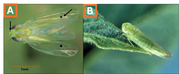
Figure 1. Cotton jassid adults (A) have one black dot on each wing and may have two small dots between their eyes (these dots on the crown can fade). The potato leafhopper (B), which is not a threat to cotton production but does occur in Oklahoma, does not have black dots on their wings or between their eyes. Image A courtesy of Isaac Esquivel, UF Extension, image B courtesy of DryBeanAgronomy.ca.
Biology and Host Range
The cotton jassid has a short life cycle, completing a generation in approximately two weeks under warm conditions.
- Reproduction: Eggs are inserted directly into leaf midveins and petioles, hatching in 3–4 days. Eggs will not be visible to the naked eye or through hand lens. Cotton jassids progress through 5 nymphal instars before becoming reproductive adults (Figure 2).
- Host Plants: This pest is polyphagous, meaning it feeds on many hosts. While cotton is a primary target, it also thrives on okra, eggplant, and ornamental hibiscus. It has also been found on native plants like Turk’s cap, as well as weeds like Ceasar weed and Florida pusley.
- 2025 Range on U.S. Cotton: The cotton jassid was detected on cotton in FL, GA, AL, MS, LA, TN, SC, NC, and TX. The TX detections in cotton were limited to southeastern TX in Grimes, Wharton, and Fort Bend counties. At the time of this article’s posting (March 2026), the cotton jassid has not been detected in OK.
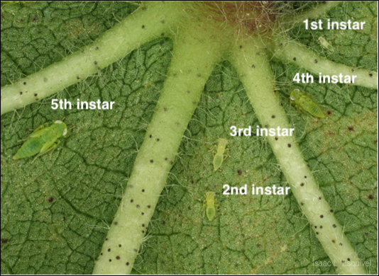
Figure 2. Cotton jassid nymphs on the underside of a cotton leaf. Image courtesy of Isaac Esquivel, UF Extension.
Damage: Recognizing Hopperburn
Unlike other leafhoppers, the cotton jassid injects a salivary toxin that disrupts the plant’s vascular system.
- Early Signs: Initial yellowing that resemble potassium deficiency with some upward curling of leaf margins (Figure 3, Rating 1).
- Progression: Characterized by hopperburn, a yellowing (chlorosis) that proceeds from leaf edges and turns red or brown as the tissue dies (Figure 3).
- Systemic Impact: Plants can go downhill quickly, often leading to complete desiccation and stunted growth (Figure 4).
A Hopperburn Injury Rating Scale has been developed by Extension Cotton Entomologists in the mid-South (Figure 3). You cannot let the cotton jassid get ahead of you. Once reddening starts on the leaf margins (Rating 2 in Figure 3) it is likely too late to rescue the cotton plant, damage will quickly progress and photosynthetic capabilities for the plant decline considerably.
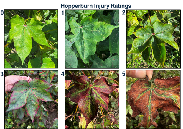
Figure 3. Hopperburn injury rating scale for cotton jassid damage. Damage increases from none (0) to severe damage of desiccated leaf (5). Slight yellowing and upward curling of leaf is shown in Rating 1, with increased yellowing, cupping, and beginnings of reddened leaf margins in Rating 2. Insecticide action should be taken prior to reaching Rating 2. Ratings 3 – 5 show increased spread of reddening and desiccation. Images courtesy of Phillip Roberts (UGA Extension) and Scott Graham (AU Extension).
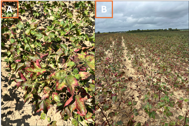
Figure 4. Cotton jassid hopperburn resulting in reddened, dried leaves (A) and stunted cotton plants (B). Image courtesy Isaac Esquivel, UF Extension.
Scouting Protocol
Scouting is mandatory for every cotton field in 2026 to prevent significant yield loss. Plants located at the edge of cotton fields can serve as good indicators, as cotton jassids will enter at field margins where damage is more likely to occur before further in field.
- Target Area: Inspect the undersides of leaves in the mid-to-upper canopy.
- Sample Leaf: Focus on the 4th mainstem leaf below the terminal, as this is where nymphs typically congregate.
- Visual Checks: Because adults fly quickly, count the flightless nymphs. Examine at least 25 leaves per field.
- Threshold: 1 cotton jassid per leaf, or early crop injury indicators (Figure 3, Rating 1) with cotton jassid confirmations nearby.
- Continue Scouting: Since green leaves are needed to fill bolls, growers should scout cotton up to at least 2 weeks prior to defoliation.
Management Guidance
Cultural Practices
- Plant Early: Trials indicate that earlier planting dates can help the crop “outrun” the peak pressure of migrating populations.
- Nutrient Management: Avoid excess Nitrogen, which attracts cotton jassids. Ensure adequate Potassium, as deficient plants crash much faster under cotton jassid stress.
- Varieties: Internationally, varieties with high trichome (hair) density on leaves offer natural resistance to feeding. However, varieties on the U.S. market are generally less hairy than those planted elsewhere. Currently, trials from 2025 do not indicate a varietal difference in terms of cotton jassid susceptibility.
Chemical Control
Based on 2025 research trials conducted by Mid-South Cotton Extension Entomologists, the following insecticides have shown varying levels of control (Table 1). Repeated insecticide applications may be warranted.
Table 1. Suggested foliar insecticides* and their observed control level for suppressing the cotton jassid. Efficacy lasted around 2 weeks.
| Control Level | Insecticides |
| High (>70% Control) | Carbine, Sefina, Sivanto, Bidrin, Venom, Plinazolin |
| Moderate (50-70%) | Transform, Centric, Assail, Orthene |
| Low (<50%) | Steward, Diamond, Bifenthrin, Admire Pro |
*Cotton jassids have shown resistance to every chemistry class in their native range; rotation of modes of action is critical. The mention, listing, or use of specific insecticides is not an endorsement of that product, nor is it a criticism of similar products not mentioned.
If you suspect cotton jassid activity or see hopperburn symptoms, contact the OSU Cotton IPM team: Maxwell Smith (maxwell.smith@okstate.edu), Ashleigh Faris (Ashleigh.faris@okstate.edu), and Jenny Dudak (jdudak@okstate.edu) immediately for confirmation. This team will be monitoring for the cotton jassid and will share updates on nearing threat, Oklahoma detections, and updated management guidance as it becomes available.
For more information on the cotton jassid in the U.S., click on this link to access Extension Factsheets, podcasts, and videos developed by Extension Entomologists managing the pest: https://drive.google.com/file/d/19IFT5c9b5JXEaBgf6X-weya07G56RXS5/view?usp=sharing.
Small Pest, Big Problems: Wheat Curl Mites and Wheat Streak Mosaic Virus Detected in Oklahoma
Ashleigh Faris, Cropping Systems Entomologist, IPM Coordinator
Meriem Aoun, Wheat Pathologist
Department of Entomology & Plant Pathology,
Oklahoma State University
Wheat Curl Mite (WCM) activity has been confirmed in Washita County, located in western Oklahoma. While the mites themselves are difficult to see, they can have a considerable impact on wheat health, primarily due to their role as vectors for several viral diseases such as wheat streak mosaic virus (WSMV). The Plant Disease and Insect Diagnostic Laboratory (PDIDL) has confirmed WSMV in the sample where WCM were detected in Washita County. This week, the PDIDL has also confirmed infection by WSMV in Blaine County (Canton, OK), McCurtain County (Garvin, OK), and Cleveland County (Noble, OK).
Identification
The Wheat Curl Mite is nearly invisible to the naked eye. At approximately 1/100 of an inch long, these pests require a 10x – 20x hand lens for proper identification.
- Appearance: They are white or cream-colored, cigar-shaped (cylindrical), and possess only four legs located near the head (Figure 1).
- Behavior: They are typically found in the protected areas of the plant, such as developing, youngest leaves or the furrows of the leaf surface. As the leaf unfurls, the mites migrate to the next emerging leaf.
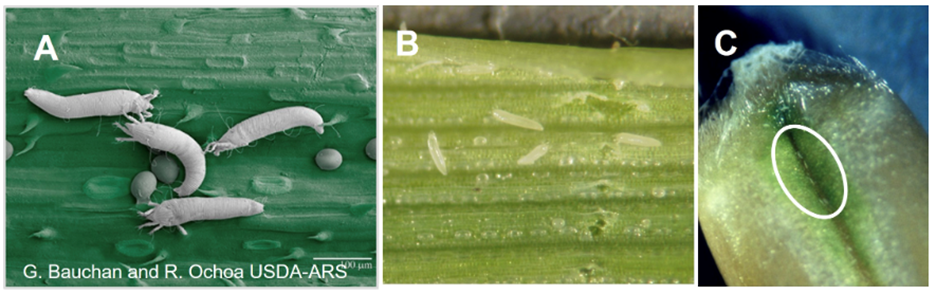
Figure 1. Wheat curl mites and eggs on a wheat leaf (A, B), and mites on a maturing wheat kernel (C). Images courtesy G. Bauchan and R. Ochoa, USDA-ARS.
Biology and Life Cycle
Understanding the WCM life cycle is critical for preventative management:
- Rapid Reproduction: Under optimal temperatures (75° – 85°F), a WCM can complete its life cycle in 7 to 10 days. This allows populations to explode rapidly during warm autumns or springs.
- Dispersal: WCMs cannot fly; they rely entirely on wind currents to move from plant to plant or field to field. They crawl to the tips of leaves and hitchhike on the wind.
- Survival (The Green Bridge): WCMs are obligate parasites, meaning they require living green tissue to survive and reproduce. They persist through the summer on volunteer wheat and various perennial or annual grasses. This is known as the green bridge. If this bridge is not broken, mites move into the newly planted crop in the fall.
Damage and Virus Transmission
WCMs cause two types of damage:
- Direct Feeding: Mites suck sap from the leaf cells. This causes the edges of the leaf to roll inward (the curl part of WCM) (Figure 2). This curling provides a protected microclimate for the mites to reproduce. Heavy infestations can cause stunting and a slowed appearance in growth.
- Viral Vector (Primary Concern): The WCM is the sole vector for Wheat Streak Mosaic Virus (WSMV), High Plains Wheat Mosaic Virus (HPWMoV), and Triticum Mosaic Virus (TriMV).
- Symptoms: Infected plants show yellowing, mottled or streaked leaves, and severe stunting (Figures 3 & 4).
- Impact: If infection occurs in the fall, yield loss can be up to 100%. Spring infections are generally less damaging.
Scouting Techniques
Because the mites are so small, scouting focuses on leaf symptoms and having a hand lens:
- Check your Fields: Examine the youngest leaves of the wheat plant. Look for the characteristic inward rolling of the leaf edges (Figure 2).
- Use Magnification: Slowly unroll a suspect leaf and use a hand lens to look for tiny, white, slow-moving specks in the leaf furrows.
- Pattern of Infestation: Wind-dispersed mite infestations often start at the edge of a field (particularly edges adjacent to volunteer wheat or CRP land) and move inward in the direction of prevailing winds. Areas with infestations may show signs of yellowing and appear as patches distributed at random across the field (Figure 4).
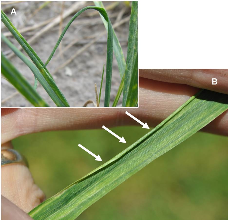
Figure 2. Infestation of wheat curl mites on wheat results in tightly curled leaves and entrapment of subsequent leaves within the curl (A). After full leaf emergence, a tight curl at the leaf edge remains (B). Images courtesy of UNL Extension.
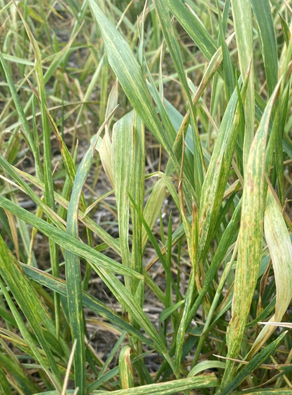
Figure 3. Wheat streak mosaic virus (WSMV) symptoms includeyellowing, mottled or streaked leaves. Image courtesy of Meriem Aoun, Oklahoma State University.
Figure 4. Plants at field margins, neighboring a wheat curl mite source, are the first to become infected with viruses of the Wheat Streak Mosaic Virus (WSMV) complex and develop symptoms, such as yellowing and streaking. Notice the gradient in color from the field edge (left) toward the center of the wheat field. Image courtesy of UNL Extension.
Management Recommendations
Currently, there are no effective rescue chemical treatments for WCM once symptoms appear in the field. Miticides generally do not reach the mites hidden inside the curled leaves. Management must be proactive:
- Manage volunteer wheat and grassy weeds: This is the most effective management tool to break the green bridge. Ensure all volunteer wheat and grassy weeds are completely dead (via tillage or herbicide) at least two weeks prior to planting the new crop. WCMs will starve within days without a living host.
- Delayed Planting: Planting wheat later in the fall reduces the window of time that mites must migrate into the crop and slows their reproduction rate as temperatures drop.
- Variety Selection: Some wheat varieties offer resistance or tolerance to WCM or WSMV. Consult the latest OSU variety trial data to select adapted varieties for north-central Oklahoma that carry these traits. Currently, Breakthrough is the most resistant OSU variety, which carries the WSMV resistance gene, Wsm1.
Brown Wheat Mite Activity in North Central Oklahoma
Ashleigh Faris, Cropping Systems Entomologist, IPM Coordinator
Department of Entomology & Plant Pathology,
Oklahoma State University
Following a period of dry weather, wheat growers in central Oklahoma are reporting activity of the Brown Wheat Mite (BWM). Unlike many other wheat pests, BWM thrives in drought conditions, and its damage can often be mistaken for moisture stress or nutrient deficiency.
Identification
The Brown Wheat Mite is small—about the size of a needle point—but is generally easier to spot than the Wheat Curl Mite because it is active on the leaf surface.
- Appearance: BWM has a dark red to brownish-black, oval-shaped body (Figure 1).
- Distinguishing Feature: Its front legs are significantly longer than its other three pairs of legs.
- Behavior: They are most active during the day, particularly in the afternoon, and will quickly drop to the ground if the plant is disturbed (Figure 2).
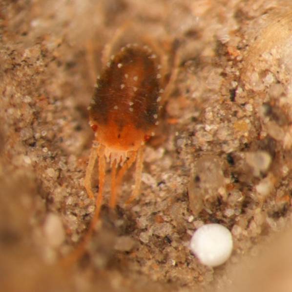
Figure 1. Brown wheat mite (BWM).
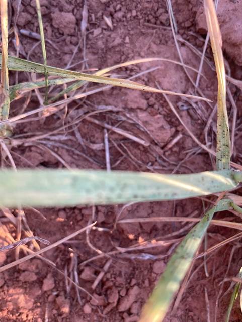
Figure 2. Brown wheat mites (BWM) on wheat. Image courtesy L. Galvin, OSU Extension.
Biology and Life Cycle
BWM populations consist entirely of females that produce offspring without mating (parthenogenesis), allowing for extremely rapid population growth under dry conditions. The BWM has a unique life cycle in that it can lay two types of eggs. Environmental conditions dictate when these two types of eggs are laid:
- Red Eggs: Laid during the growing season and hatch in about a week when conditions are favorable.
- White (Diapause) Eggs: Laid as temperatures rise and the crop matures. They are highly resistant and allow the population to survive the summer heat, hatching only when cooler, wetter weather arrives in the fall.
Damage
BWM damage is caused by the mites piercing plant cells and sucking out the plant nutrients.
- Symptoms: Initial damage appears as “stippling” (fine white or yellow spots) on the leaves. As feeding continues, leaves take on a silvery or bronzed appearance (Figure 3).
- Tipping: Heavy infestations cause the tips of the leaves to turn brown and die.
- Weather Interaction: Damage is most severe when plants are already under drought stress. Because both BWM damage and drought cause yellowing/browning, it is essential to confirm the presence of mites before treating.
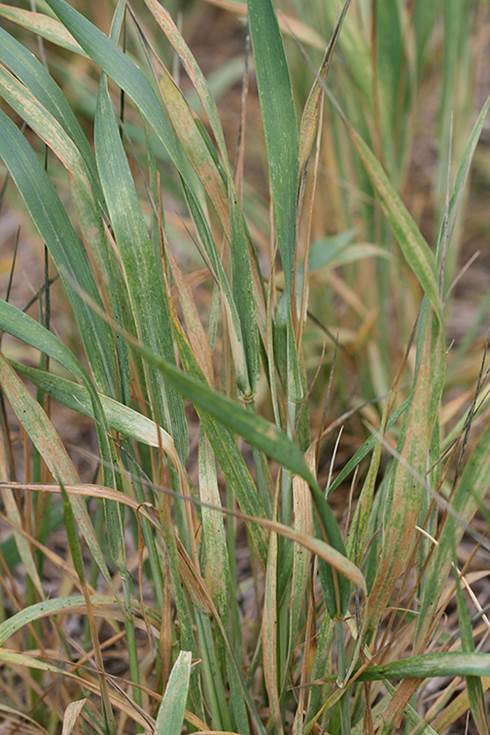
Figure 3. Brown wheat mite (BWM) damage.
Scouting
Because BWM is highly mobile and drops when disturbed, careful scouting is required:
- Timing: Scout during the warmest part of the day when mites are most active on the upper leaves.
- The Paper Test: Gently but quickly shake or tap wheat plants over a white piece of paper or a white clipboard. Look for tiny dark specks moving across the surface.
- Economic Threshold: While thresholds vary based on crop value and moisture stress, research suggests a treatment threshold of 25 to 50 brown wheat mites per leaf in wheat that is 6 inches to 9 inches tall is economically warranted. An alternative estimation is “several hundred” per foot of row. If the wheat is severely stressed, the lower end of that threshold should be used.
Management Recommendations
- The “Rain” Factor: A significant, driving rain is often the most effective control for BWM. Rain can physically knock mites from the plant and promote fungal pathogens that naturally reduce the population.
- Chemical Control: If populations exceed the threshold and no rain is in the forecast, chemical intervention may be necessary. Know the cost of the treatment and value of your wheat so you can determine if an application is a worth return on investment.
- Effective Ingredients: Organophosphates (such as Dimethoate) have historically provided better control than many pyrethroids, as the latter can sometimes result in mite “flaring” or simply fail to provide adequate residual control.
- Coverage: High water volume is critical to ensure the insecticide reaches the mites, especially if they have moved toward the base of the plant.
- Pre-harvest Intervals & Grazing Restrictions: Always read and follow the label guidelines. For more on acaricides that can be applied in wheat see the Oklahoma State University Fact Sheet “Management of Insect and Mite Pests in Small Grains” (CR-7194).
- Cultural Practices: Since BWM thrives in dry, dusty conditions, maintaining good soil moisture and vigorous plant growth can help the crop tolerate feeding. Here’s to hoping for some rain soon in the forecast; we could really use it for lots of reasons in Oklahoma.
Corn Hybrids’ Yield Response to Limited Well Capacities in the Central High Plains
Macie McPeak: M.S in Irrigation and Water Management
Sumit Sharma : Extension Specialist for High Plains Irrigation and Water Management
Background
The Central High Plains, which include the Oklahoma Panhandle, Southwest Kansas, Southeast Colorado, and Northern Texas Panhandle, is a heavily farmed semi-arid region that depends on the Ogallala Aquifer for irrigation to ensure stable crop yields. However, the continuous decline of the Ogallala Aquifer has resulted in increased need for irrigation strategies that conserve water while maintaining crop profitability. Corn remains the most water consuming crop with highest productivity per unit of irrigation applied, and strong economic returns in the Central High Plains region. However, corn is also the most sensitive to water stress among all the existing cropping systems (including sorghum, cotton, and sunflower, soybeans and wheat). Declining water table has reduced the well capacities in many areas in the region, which cannot meet crop water demand, making it a growing challenge for corn production. Therefore, there is a need for research in irrigation strategies and agronomic choices such as drought tolerant hybrids, seeding rate, planting date, and hybrid maturity for sustainable and profitable corn production with reduced well capacities in the region. This blog discusses the yield response of different corn hybrids to limited well capacities in the Oklahoma Panhandle area of the Central High Plains.
Limited well capacities only meet partial crop water demand, which in general leads to yield declines especially in high water demanding crops such as corn. Several previous studies suggest that crop productivity does not significantly decrease as long as irrigation is maintained at approximately 75–80% of full evapotranspiration (ET) replacement (Su et al., 2022; Klocke et al., 2007; Zhao et al., 2019). However, when irrigation levels are more restricted, such as under reduced well capacities, there can be substantial yield losses and diminished economic returns. The magnitude of yield reduction varies with region, hybrids, and growth stage at which water stress occurred. For example, in the Central High Plains the corn ET demand is highest in Texas Panhandle and decreases as we move north towards Nebraska. Zhao et al. (2019) found that applying 75% ET in the Texas Panhandle produced corn yields equivalent to full irrigation, whereas reducing irrigation to 50% caused significant yield reductions. Similarly, Klocke et al. (2007) reported that limited irrigation at roughly 50% of full ET replacement in Nebraska achieved 80–90% of fully irrigated yields across multiple crop rotations. Therefore, the irrigation strategies which work in one region may not work the same way in other regions with different crop water demand and must be tested for the region-specific climatic conditions.
The current study was conducted in 2025 at the Oklahoma Panhandle Research and Extension Center in Goodwell, OK. Four Pioneer brand corn hybrids including P13777 (113 day maturity), P10625 (110 day maturity), P05810 (105 day maturity), and P14346 (114 days maturity) were planted at 22,000 and 28,000 seeds per acre. The hybrids were irrigated with a center pivot fitted with variable rate irrigation system at 200, 300, 400, and 500 GPM well capacities. The well capacities were simulated by adjusting the frequency of irrigation events.
Results & Discussion
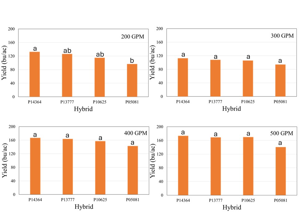
The crop received 12.1 inches of rain from planting until physiological maturity, while total rainfall from April till September was over 15 inches. Manual probing of the field showed near 4 feet soil profile at the time of planting which can hold up to 2 inches of plant available water per foot. The well capacities 200, 300, 400, and 500 GPM treatments received 7.4, 8.9, 10.8, and 12.0 inches of irrigation, respectively. The data showed no significant effect of population on corn yield across hybrids for any well capacity. However, the hybrids showed significant interaction with well capacities, which indicated that hybrid yield response varied at different capacities (Figure 1). In general, the average yield declined from longest maturity to shortest maturity hybrids irrespective of the well capacity, but was only statistically significant at for 200 GPM (Figure1). At this irrigation level, the shortest maturity hybrid P05081 yielded significantly lower yield than longest maturity hybrid P14364, while P13777 and P10625 were not different from either of these two hybrids.
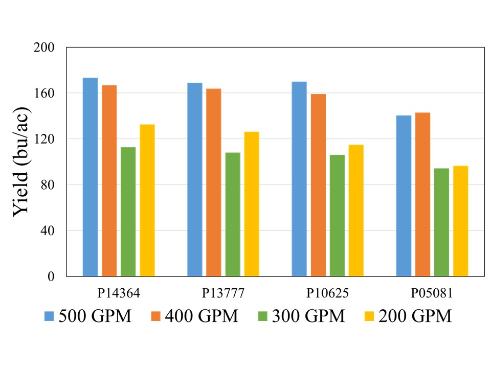
Although there was no statistical difference among the hybrids at 500, 400, and 300 GPM, when compared across well capacities, yield reductions were most pronounced at the 200 and 300 GPM irrigation levels for each individual hybrid, indicating that irrigation capacity was the primary yield limiting factor under restricted water availability (Figure 2). While the exact causes of this abrupt decline are not yet understood, as mentioned in the beginning of this blog, previous literature has suggested that severe yield decline in corn can be expected when irrigation is reduced to 60% ET replacement in the study region. Both 300 and 200 GPM well capacities met 60 and 65% crop ET demand, while 400 and 500 GPM met 71 and75% crop ET demand, respectively. More data will be needed to ascertain these threshold levels of well capacities for corn production in this region.
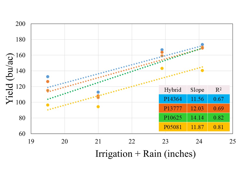
All the hybrids showed a positive yield response to Irrigation+Rain with different yield gains per inch of water applied (Figure 3). Hybrid P10625 registered highest yield gain of 14.1 bushel per inch of water applied, followed by P13777 (12.0 bu), P05081 (11.9 bu), and P14364 (11.6 bu). The stronger coefficient of regression (>80%) for two short maturity varieties indicated that irrigation was stronger yield limitation factor for these hybrids, in comparison to 114 and 113-day maturity hybrids for irrigation explained on 67 and 69% variability, respectively. This suggests that besides irrigation there might be other factors which could contribute to filling the yield gaps for given irrigation levels in longer maturity hybrids.
Planting population did not significantly affect grain yield across irrigation capacities. When pooled across the hybrids for individual planting populations, 28,000 seeding rates resulted in gain of 0.1, 2.6, 5, and 12 bushels per acre for 200, 300, 400, and 500 GPM, respectively. This indicates that higher planting populations at well capacities of 400 or above should be considered, while reducing population at 300 GPM or lower might be more cost-effective option.
Take Home
- Irrigation capacity remains the primary determinant of yield potential under limited well capacities in the Central High Plains.
- Pre-irrigation and recharging the soil profiles will be critical to support crop water demand for limited well capacities.
- Short maturity hybrids appeared to have consistently lower average yield and more vulnerable for yield losses at limited irrigation. However, one must consider that the growing conditions were more conducive for corn production in 2025 which generally favor long maturity hybrids. Therefore, long-term data will be required to assess the performance of short maturity hybrids during inclement growing seasons.
- Even though population didn’t significantly influence the grain yield. The 28,000 seeding rates overall had higher average yield at 400 and 500 GPM. Therefore, producers should consider the higher population at these well capacities or more.
- Overall, irrigation is the most important factor for yields, but there is a need for long-term agronomic data on hybrid maturity and population along with economic analysis to ascertain these findings.
Check Your Wheat: Greenbugs Reported in Central Oklahoma
Ashleigh M. Faris
Cropping Systems Extension Entomologist
Department of Entomology & Plant Pathology
Oklahoma State University
Wheat producers in central Oklahoma are reporting the presence of the greenbug, Schizaphis graminum, in winter wheat fields. Greenbugs are one of the most important insect pests of wheat in the southern Great Plains and can occur from fall through spring. These aphids feed on plant sap and inject toxins into wheat plants, causing characteristic leaf discoloration and plant injury.
Early detection through field scouting is essential to determine whether populations are increasing and if an insecticide treatment is justified.
Greenbug Identification & Biology
Key identifying characteristics of greenbug (Figure 1):
- Small aphids (~1/16 inch long)
- Pale to lime-green body
- Dark green stripe down the middle of the back
- Dark tips on antennae and legs
- Found in colonies on the underside of wheat leaves
Greenbugs reproduce rapidly under favorable conditions (between 55° F and 95° F) and often occur in patches within fields rather than evenly distributed populations. During periods of cool weather, the greenbug may increase to enormous numbers, due to the absence of natural enemies, which develop significantly slower compared to greenbugs at such temperatures. On the other hand, cold weather can also influence aphid populations. However, this latest cold snap is not enough to eliminate greenbugs. It takes average temperatures below 20° F for at least a week to kill a substantial number of greenbugs in wheat.
Greenbug Damage in Wheat
Greenbugs damage wheat in two ways, through direct feeding and injection of toxic saliva. Greenbugs may also transmit barley yellow dwarf virus (BYDV), which can further reduce yield potential.
Typical early symptoms include small, reddish or copper spots on leaves (Figure 2) and yellowing around feeding sites. Advanced infestations will result in leaves turning yellow or orange, dead leaf tissue, stunted plants, and expanding patches of dead wheat. Heavy infestations may kill seedlings and reduce tillering, particularly during drought stress.

How to Scout for Greenbugs
The Glance-N-Go™ sampling system developed by Oklahoma State University can help determine whether aphid populations exceed economic thresholds. Download the Greenbug Glance N’ Go Sampler app for your smartphone. You will then input the control cost ($/Acre), crop value ($/Acre), and the Spring sampling window. Use a zig-zag or W-pattern (Figure 3) to scout your field, checking undersides of leaves at three tillers per stop for greenbugs and brown mummies. Use the app to record the numbers of these insects and sample until the app tells you to stop sampling or tells you treat. As temperatures warm, continue to scout regularly as greenbug populations may build.

Scouting recommendations without the Greenbug Glance N’ Go Sampler app:
- Walk a W or zigzag pattern across the field.
- Examine 10–20 plants at each stop.
- Check:
- Underside of leaves
- Leaf midrib
- Base of tillers
- Record:
- Aphids per tiller
- Presence of aphid mummies (Figure 4)
- Beneficial insects
Beneficial Insects
Natural enemies frequently control aphid populations. While scouting for greenbug you should also look for lady beetles, lacewing larvae, hoverfly larvae, and parasitized aphids (“mummies”) (Figure 4). If beneficial insects are abundant, aphid populations may decline without insecticide treatment. Where there are one to two lady beetles (adults and larvae) per foot of row, or 15 to 20 percent of the greenbugs have been parasitized, control measures could be delayed until it is determined whether the greenbug population is continuing to increase.
Based on current wheat scouting, it appears that parasitoid numbers are low this 2026 season so continuing to scout for greenbug will be critical in responding to populations that go unchecked by beneficials.
Economic Threshold Guidelines
The simplest way to determine if action needs to be taken against greenbugs is to utilize the Glance-N-Go™ sampling system developed by Oklahoma State University. Approximate guidelines historically used in Oklahoma wheat can be found in Table 1 below.

Thresholds are influenced by:
- Wheat growth stage
- Crop value
- Cost of treatment
- Presence of beneficial insects
Insecticides Labeled for Greenbugs in Wheat
Aphid feeding and insecticide performance are strongly influenced by temperature. Greenbugs tend to move higher on wheat plants during warm conditions but may move lower on the plant or below ground during cold weather, reducing exposure to insecticides. As a result, damaging populations are most often observed in late winter and early spring. Insecticides generally perform best when temperatures are above 50°F, and control may occur more slowly in cooler conditions (e.g., control at 45° F may take roughly twice as long as at 70° F). If applications must be made under cooler temperatures, use the highest labeled rate. Wheat grown under irrigation can typically tolerate higher greenbug populations than dryland wheat.
Always follow pesticide label directions, application sites, and rates. Be sure to read and follow the label for preharvest intervals (PHI) and restricted-entry intervals (REI). Use a minimum of 10 GPA by ground and 3 GPA by air (if labelled for aerial application) to ensure adequate coverage.
For assistance with aphid identification or treatment decisions, see OSU Fact Sheet EPP-7099 Small Grain Aphids in Oklahoma and Their Management, or contact your local OSU Extension office.
Thoughts from an Agronomist- 1 Management of the Primordia
Josh Lofton, Cropping Systems Specialist
Many crop management recommendations emphasize actions that must be taken well before a crop reaches what we often call “critical growth stages.” Management this early can seem counterintuitive when the crop still looks small, healthy, or unchanged aboveground. However, much of a crop’s yield potential is determined early in the season at a level we cannot see in the field. Long before flowers, tassels, or heads (or any reproductive structure) appear, the plant is already making developmental decisions that shape its final yield potential. Understanding this “behind the scenes” process helps explain why timely, early-season management is often more effective than trying to correct problems later.
At the center of this process is the shoot apical meristem, commonly referred to as the growing point. This tissue produces leaf and reproductive primordia, which are the earliest developmental stages of future everything in the plant. These primordia form well before the corresponding plant parts are visible. Once these structures initiate—or if they fail to begin due to stress—the outcome is permanent. The plant cannot later in the season go back and recreate leaf number, leaf size, or reproductive capacity. As a result, early environmental conditions and management decisions play a disproportionate role in determining yield potential.
Corn is a good example of how early development influences final yield. By the time corn reaches the V4 growth stage, the plant only has four visible leaves with collars, yet internally it is far more advanced. Most of the total leaf primordia that will eventually form the full canopy have already begun, and the potential size of the ear is starting to be established. During this stage, the growing point is still below the soil surface and somewhat protected from some stressors but highly susceptible to others. Nitrogen deficiency, cold temperatures, moisture stress, compaction, or herbicide injury at or before V4 can reduce leaf number and limit leaf expansion. Even if growing conditions improve later, the plant cannot replace leaf primordia that were never formed, which reduces its ability to intercept sunlight and support high yields.
As corn approaches tasseling (VT), the crop enters a stage that is visually and physiologically important. Pollination, fertilization, and early kernel development occur at this time, and stress can have a critical impact on kernel set. However, by VT, the plant has already completed leaf formation, and much of the ear size potential has already been determined several growth stages earlier. Management at VT is therefore focused on protecting yield rather than creating it. Late-season nutrient applications may improve plant appearance or maintain green leaf area, but they cannot increase leaf number or rebuild ear potential lost due to early-season stress. This distinction helps explain why some late inputs show limited yield response even when the crop looks responsive.
Grain sorghum provides another clear example of why early management is emphasized. Although sorghum often grows slowly early in the season and may appear unimportant during the first few weeks after emergence, the first 30 days are among the most critical periods in its development. During this time, the growing point is actively producing leaf primordia and transitioning from vegetative growth toward reproductive development. Head size potential is primarily established during this early window, and the plant’s capacity to support tillers is influenced by early nutrient availability and moisture conditions. Stress from nitrogen deficiency, drought, weed competition, or restricted rooting during the first 30 days can reduce head size and kernel number long before visible symptoms appear.
Once sorghum reaches later vegetative and reproductive stages, much like corn at VT, management shifts from building yield potential to protecting what has already been determined. Improving conditions later in the season can help maintain plant health and grain fill, but it cannot fully compensate for early limitations imposed at the primordial level. This is why early fertility placement, timely weed control, and moisture conservation are consistently emphasized in sorghum production systems.
Across crops, a typical pattern emerges: the growth stages we observe in the field often reflect decisions the plant made weeks earlier. When agronomists stress early-season management, they are responding to plant biology rather than simply following tradition. By the time visible “critical stages” arrive, the plant has already established many of the components that define yield potential.
The key takeaway is that effective crop management must be proactive rather than reactive. Early-season decisions support the crop while it is still determining how many leaves it can produce, how large its reproductive structures can become, and how much yield it can ultimately support. Waiting until stress becomes visible often means responding after the plant has already adjusted its potential downward. Recognizing what is happening at the primordial level helps explain why management ahead of critical stages consistently delivers the greatest return, even when the crop appears small and unaffected aboveground.
For questions or comments reach out to Dr. Josh Lofton
josh.lofton@okstate.edu
One Well-Timed Shot: Rethinking Split Nitrogen Applications in Wheat production
Brian Arnall, Precision Nutrient Management Specialist
Samson Abiola, PNM Ph.D. Student.
Nitrogen is the most yield limiting nutrient in wheat production, but it’s also the most unpredictable. Apply it too early, and you risk losing it to leaching or volatilization before your crop can use it. Apply it too late, and your wheat has already determined its yield potential; you’re just feeding protein at that point. For decades, the conventional wisdom has been to split nitrogen applications: put some down early to get the crop going, then come back later to apply again. But does splitting actually work? And more importantly, when is the optimal window to apply nitrogen if you want to maximize both yield and protein quality? We spent three years across different Oklahoma locations testing every timing scenario to answer these questions.
How We Tested Every Nitrogen Timing Scenario in Oklahoma Wheat
Between 2018 to 2021, we conducted field trials at three Oklahoma locations, including Perkins, Lake Carl Blackwell, and Chickasha, representing different soil types and growing conditions across the state. We tested three nitrogen rates: 0, 90, and 180 lbs N/ac, applied as urea at five critical growth stages based on growing degree days (GDD). These timings were 0 GDD (preplant, before green-up), 30 GDD (early tillering), 60 GDD (active tillering), 90 GDD (late tillering, approximately Feekes 5-6), and 120 GDD (stem elongation, approaching jointing). We also compared single applications at each timing against split applications, where half the nitrogen (45 lbs N ac-1) went down preplant, and the other half was applied in-season (45 lbs N ac-1).
The Sweet Spot: Yield and Protein at the 90 lbs N/ac Rate
Across all site-years, at the 90 lbs N/ac rate, timing had a significant impact on both yield and protein. The highest yields came from the 30 and 90 GDD timings, producing 62 to 66 bu/ac, with 60 GDD reaching the peak (Figure 1). Protein at these early timings stayed relatively modest at 13%. The 90 GDD timing delivered 62 bu/ac with 14% protein matching the yield of the 30 GDD application but pushing protein a percentage higher (Figure 2). The real problem appeared at 120 GDD. Delaying application until stem elongation dropped yields to just 49 bu/ac, even though protein climbed to 15%. That’s a 13 bushel penalty compared to the 90 GDD timing. At current wheat prices per bushel, that late application may cost farmers over $100 per acre in lost revenue. By 120 GDD, the crop has already determined its yield potential tillers are set, head numbers are locked in and nitrogen applied at this stage can only be directed toward protein synthesis, not building more yield components.
More Nitrogen Does not lead to high yield
Doubling the nitrogen rate to 180 lbs N/ac revealed something critical, more nitrogen doesn’t mean more yield. The yield pattern remained nearly identical to the 90 lbs N/ac rate. The 60 GDD timing produced the highest yield at 68 bu/ac, followed closely by 30 GDD at 67 bu/ac. The 90 GDD timing yielded 62 bu/ac, and the 120 GDD timing again crashed to 51 bu/ac. The only difference between the two rates was protein concentration (Figure 2). At 180 lbs N/ac, protein levels increased across all timings: 13% at preplant, 15% at both 30 and 60 GDD, 15-16% at 90 GDD, and 16% at 120 GDD. This confirms a fundamental principle: once farmers supply enough nitrogen to maximize yield potential, which occurred at 90 lbs N/ac in these trials, additional nitrogen only increases grain protein. It does not build more bushels. Unless farmers are receiving premium payments for high-protein wheat, that extra 90 lbs of nitrogen represents a cost with no yield return.

Should farmers split their nitrogen application?
Now that timing has been established as critical, the next question becomes: should farmers split their nitrogen applications, or is a single application sufficient? The conventional recommendation has been to split nitrogen apply part preplant to support early growth and tillering, then return with a second application later in the season to boost protein and finish the crop. But does the data support this practice? We compared three strategies at each timing: applying all nitrogen preplant, applying all nitrogen in-season at the target timing, or splitting nitrogen equally between preplant and in-season timing. The goal was to determine whether the extra trip across the field will deliver better results.
Our findings revealed that splitting provided no consistent advantage. At 30 GDD, all three strategies preplant, in-season, and split performed identically, producing 62-65 bu/ac with 12-13% protein (Figure 3 and 4). No statistical differences existed among them. At 60 GDD, similar pattern was held. Yields ranged from 61 to 66 bu/ac and protein stayed at 12-13% regardless of whether farmers applied all nitrogen preplant, all at 60 GDD, or split between the two. At 90 GDD, the single in-season application actually outperformed the split. While yields remained similar across all three methods (61-64 bu/ac), the in-season application delivered significantly higher protein at 13.7% compared to 12.4% for preplant and 12.5% for split applications. This suggests that concentrating nitrogen at 90 GDD, rather than diluting it across two applications, allows more efficient incorporation into grain protein. The only timing where splits appeared beneficial was 120 GDD, where the split application yielded 59 bu/ac compared to 51 bu/ac for the single late application. But this is not a win for splitting, it simply demonstrates that applying all nitrogen at 120 GDD is too late and putting half down earlier salvages some of the yield loss. Across all timings tested, splitting nitrogen into two applications offered no agronomic advantage over a single well-timed application, meaning farmers are making an extra pass for no gain in yield or protein.


Practical Recommendations for Nitrogen Management
Based on three years of field data, farmers should target the 90 GDD timing (late tillering, Feekes 5-6) for their main nitrogen application to achieve the best balance between yield and protein. This window typically falls in late February to early March in Oklahoma, though farmers should monitor crop development rather than relying solely on the calendar apply when wheat shows multiple tillers, good green color, and vigorous growth. A rate of 90 lbs N/ac maximized yield in these trials; higher rates only increased protein without adding bushels, so farmers should only exceed this rate if receiving premium payments for high-protein wheat. Splitting nitrogen applications provided no advantage at any timing, meaning a single well-timed application at 90 GDD is sufficient for most Oklahoma wheat production systems. The exception would be sandy soils with high leaching potential, where splitting may reduce nitrogen loss. Farmers should avoid delaying applications until 120 GDD or later, as this timing consistently resulted in 15-25 bushel per acre yield losses even though protein increased. For farmers specifically targeting premium protein markets, a two-step strategy works best: apply 90 lbs N/ac at 90 GDD to establish yield potential and baseline protein, then follow with a foliar application of 20-30 lbs N/ac at flowering to push protein above 14% without sacrificing yield. Finally, weather conditions matter hot, dry forecasts increase volatilization risk and reduce uptake efficiency, so farmers should consider moving applications earlier if low humidity conditions are expected.
Split Application Caveat * Note from Arnall.
The caveat to the it only takes one pass, is high yielding >85+ bpa, environments. In these situation I still have not found any value for preplant nitrogen application. I have seen however a split spring application is valuable. Basically putting on 30-50 lbs at green-up, with the rest following at jointing (hollowstem). The method tends to reduce lodging in the high yielding environments.
This work was published in Front Plant Sci. 2025 Nov 6;16:1698494. doi: 10.3389/fpls.2025.1698494
Split nitrogen applications provide no benefit over a single well timed application in rainfed winter wheat
Another reason to N-Rich Strip.
Yet just one more data set showing the value of in-season nitrogen and why the N-Rich Strip concept works so well.
Questions or comments please feel free to reach out.
Brian Arnall b.arnall@okstate.edu
Acknowledgements:
Oklahoma Wheat Commission and Oklahoma Fertilizer Checkoff for Funding.
Using soil moisture trend values from moisture sensors for irrigation decisions
Sumit Sharma, Extension Specialist for High Plains Irrigation and Water Management
Kevin Wagner, Director, Oklahoma Water Resources Center
Sumon Datta, Irrigation Engineer, BAE.
Sensor based and data driven irrigation scheduling has gained interest in irrigated agriculture around the world, especially in semi-arid areas because of the easy availability of commercial irrigation scheduler technology such as soil moisture sensors and crop models. Moisture sensing has particularly gained interest among the agriculture community due to ease of availability of the sensors to the producers, affordable costs, and easy to use graphical user interface. Economic potential of sensors in saving irrigation costs, data interpretation training through extension education programs, and policy initiatives have also helped with adoption of the sensors, especially in the United States. However, sensor adoption and efficient use can still be challenging due to poor data interpretation, steep learning curves, overly high expectations and subscription costs. This blog briefly discusses scenarios where sensors can be helpful in irrigated agriculture. For moisture sensor types, functioning and installation, readers are referred to BAE-1543 OSU extension factsheet.

Irrigation Scheduling
Irrigation scheduling with soil moisture sensors follows traditional principles of field capacity (FC), plant available water, maximum allowable depletion (MAD), and permanent wilting point (PWP). Figure 1 shows the transition of soil moisture level from field capacity to MAD, and to permanent wilting point in a typical soil. The maximum amount of water that a soil can hold after draining the excess moisture is called field capacity. At this point, all the water in soil is available to the plants. As the moisture content in the soil declines, it becomes more difficult for the plants to extract moisture from the soil. The soil moisture level below which the available moisture in soil cannot meet the plant’s water requirement is called the MAD. The water stress that occurs once moisture level goes below this moisture level can cause yield reductions in crops. Therefore, irrigation should be triggered as soon as the soil moisture level approaches this point (MAD) to avoid any yield losses (for detailed information on MAD, its value for different soils and crops, and irrigation scheduling, readers are referred to BAE-1537). Modern soil moisture sensors can come self-calibrated and are equipped with water stress threshold levels for different crops to avoid water stress or overwatering (Figure 2). These decisions are useful in furrow and drip irrigation systems where irrigation triggers can be synchronized with MAD values.


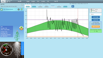
Figure 2: Screenshots of graphic user interface of three sensors a) GroGuru b) Sentek c) Aquaspy (Top to bottom) with threshold levels for soil moisture conditions. Aquspy and Sentek credits: Sumit Sharma. GroGuru image credits: groguru.com
Soil Moisture Trends and Irrigation Depths
Soil moisture sensors can help make data-informed decisions about scheduling irrigation. Previous studies have shown that the moisture values may vary from one sensor to the other and may not represent the exact moisture levels in soil. However, all soil moisture sensors exhibit trends in recharge and decline in soil moisture conditions. These real time soil moisture trends can be used to make informed decisions to adjust irrigation and improve water use efficiency. In high ET demand environments of Oklahoma, pivots are usually not turned off during the peak growing season, yet sensors can help in making decisions for early as well as late growing periods.
One of the easiest adjustments that could be made using soil moisture sensor data is the adjustment of irrigation depth. In an ideal situation, every irrigation event should recharge the soil profile to field capacity; however, this is often limited by the crops’ water demand and the well/irrigation capacity to replenish soil moisture levels. Each peak in soil moisture detected by sensors shows irrigation or rain, which ideally should be bringing moisture to same level after irrigation. However, reduction in moisture peaks in the soil moisture profile with every irrigation often indicates greater crop water demand than what is replenished with irrigation. In such scenarios, as allowed by capacity and infiltration rates, the irrigation depth can be increased. These trend values are particularly useful for center pivot irrigation systems, where triggering irrigation based on MAD might lag due to time and space bound rotations of the pivots in Oklahoma weather conditions.

Figure 3: A screenshot from Aquaspy agspy moisture sensor showing moisture at 8” (blue) and 28” (red) with each irrigation event. Data and image credit: Sumit Sharma
Last irrigation can be a tricky decision to end the cropping season. For summer crops, this is the time when crop ET demand is declining due to decline in green biomass and cooler weather patterns. Similar moisture trends can be used to make decisions for the last irrigation events, which can be skipped or reduced if the profile moisture is good, or can be provided if profile moisture is low. This is important because in an ideal situation, one would want to end the season with a relatively drier profile to capture and store off-season rains. Additionally, saving water on last irrigation can save operational cost and potentially cover the cost of moisture sensor subscriptions.
These decisions can be illustrated with Figure 3, which shows the trends of declining and recharging in a soil profile under corn at 8- and 28-inch depth. This field was irrigated with a center pivot irrigation system which was putting 1-1.25 inches of water with each irrigation event; however, the peak water recharge rate at both depths was declining with each irrigation. This coincided with peak growth period indicating rising ET demand of the crop than what was replenished by the irrigation. Later, two rain events, in addition to irrigation, replenished soil moisture in both layers. As the pivot was already running at a slow speed, slowing it further was not an option without triggering runoff for this soil type and this well capacity. Further in the season, when the crop started to senesce and ET demand declined, each irrigation event added to the moisture level of the soil. This allowed the producer to shut down the pivot between 70% starch line and physiological maturity for the crop to sustain at a relatively wet soil profile and leave the soil in relatively drier profile for the off-season.
In high ET demanding conditions of Western Oklahoma, crops often rely on moisture stored in deep soil profiles during the peak ET period when well capacities can’t keep up with crop water demand. In the high ET demanding environments of Oklahoma, irrigated agriculture depends heavily on profile moisture storage. Declining soil profile moisture is common during peak ET periods in high water demanding crops such as corn. These observations are useful if one starts the season with considerable moisture in the soil profile, however such trends may be absent if the season is started with a dry soil profile. Dry soil profiles can be recharged early in the season with pre-irrigation or deeper early irrigations (if allowed by the infiltration rate of the soil), when crop ET demand is low, to build the soil moisture profile. As such, sensors can be used in reducing the irrigation depth or skipping irrigation in early cropping systems if one starts with a full profile. This usually allows root growth through the profile to chase the moisture in deeper layers. It should be noted that the roots will grow and chase moisture only if there is a wet profile, and not through a dry soil profile.
Sensor installation and calibration are important for efficient use of these devices in irrigation decision making. Poor installation can often lead to poor data and wrong decision making. Although modern sensors are self/factory calibrated, some do provide the option to adjust threshold levels manually based on field observations. Early installation of sensors can be useful in making informed decisions as soon as the season starts. For a more detailed analysis of proper sensor installation, refer to BAE-1543. Producers are encouraged to integrate other means of irrigation planning with soil moisture sensing, such as a push rob to probe the soil profile or OSU Mesonet’s irrigation planner to further validate the sensor data. Further, the cliente should consider their irrigation capacities before investing in soil moisture sensors, as sensors may always show a deficit in low well capacities which cannot meet crop’s water demand.
References:
Taghvaeian, S., D. Porter, J. Aguilar. 20221. Soil moisture-sensing systems for improving irrigation scheduling. BAE-1543. Oklahoma State Cooperative Extension. Available at: https://extension.okstate.edu/fact-sheets/soil-moisture-sensing-systems-for-improving-irrigation-scheduling.html
Datta, S., S. Taghvaeian, J. Stivers. Understanding soil water content and thresholds for irrigation management. BAE-1537. Oklahoma State Cooperative Extension. Available at: https://extension.okstate.edu/fact-sheets/understanding-soil-water-content-and-thresholds-for-irrigation-management.html
For more information please contact Sumit Sharma sumit.sharma@okstate.edu
